
A Novel Approach for Multi-Period Reverse Logistics Network Design under High Uncertainty
- DOI
- 10.2991/ijcis.2017.10.1.77How to use a DOI?
- Keywords
- Cloud based design optimization; reverse logistics; uncertainty; network design; mixed integer programming
- Abstract
In this paper, a multi-period multi-echelon reverse logistics network design problem under high extent of uncertainty is addressed. We first formulate and then solve the multi-period network design model using the cloud-based design optimization framework which ensures to: (1) handle high number of uncertain factors; (2) propose alternative solution to traditional approaches; (3) provide a robust solution which strengthens decision makers against unexpected situations. Finally, applicability of the presented approach is tested through a dataset of e-waste reverse logistics network.
- Copyright
- © 2017, the Authors. Published by Atlantis Press.
- Open Access
- This is an open access article under the CC BY-NC license (http://creativecommons.org/licences/by-nc/4.0/).
1. Introduction
One of the most popular definitions of RL is suggested by The European Working Group on Reverse Logistics (REVLOG) as the following1: “The process of planning, implementing and controlling backward flows of raw materials, in process inventory, packaging and finished goods, from a manufacturing, distribution or use point, to a point of recovery or point of proper disposal”. The most important reason for the increased attention to RL is environmental obligations. Many regulations have been implemented which impose vital responsibilities on the actors such as original equipment manufacturers (OEMs), governmental institutions, logistics service providers, and municipalities. For instance, European Union (EU) Directives 2002/96/EC2 and 2002/95/EC3 are two of the most stringent regulations regarding the waste of electrical and electronic equipment (WEEE) (European Parliament and of the Council, Directive 2002/96/EC and 2002/95/EC 2002). The Directive contains strict obligations and quotas to reduce utilization of dangerous materials and to increase the recovery of electrical and electronic WEEE. For different periods, the Directive forces actors to collect and recover WEEE in specific amounts.
One of the research topics in the RL field is the RL network design (RLND) which has a strategic role in supply chain improvement such as the profitability and compatibility to the directives of collecting used products.4 RLND plays a role in making strategic decisions that lead to costly and critical decisions such as determination of flowing amount, location of facilities, and facility capacities.
Uncertainty is one of the basic characteristics of RLND decisions. The difficulty in representing the real-life reverse logistics problems as models and acquiring the related data includes the high uncertainty in quantity, quality, and time of product returns. Randomness and epistemic uncertainty are two types of uncertainty.5 Stochastic programming models are proposed to contend with randomness uncertainties.6,7,8 Stochastic programming can be found as weak when dealing with linguistic situations. Therefore, it is necessary to use fuzzy set theory and possibility theory9 in linguistic uncertainties such as Refs. 10–14.
Besides these approaches, there is a new model named as cloud based design optimization (CBDO) which mediates between aspects of stochastic and fuzzy programming.15 In CBDO, high uncertainty is reduced via cloud constraint. Advantages of CBDO can be summarized as following: (1) Both of certain and uncertain factors can be tackled by CBDO simultaneously; (2) CBDO’s principle is not depending on fuzziness or stochasticity, it proposes alternative solution to such kind of traditional methods, and (3) it strengthens decision makers against unexpected events. Although it is stated that the results of the proposed model are deemed satisfactory, there is a lack of applications. The contribution of this study is mainly to provide an alternative way to address the weaknesses of traditional optimization models (such as spending so much time to adopt steps etc.) by utilizing CBDO. Under these circumstances, this study proposes a CBDO model for the multi-period RLND problem and contributes to the extant literature by handling a high number of different uncertain factors of RLND in a CBDO model.
The proposed approach is designed to be used by one of the largest electric and electronic recycling firm in Turkey to restructure their RL networks for different periods under high uncertainty. We address the issue with a reverse logistics problem but not a closed loop supply chain problem because the company planned to execute the reverse product flow operations separate from the forward supply chain. The study is organized as follows: Section 2 briefly summarizes the relevant literature. The cloud-based design optimization fundamentals are reviewed in Section 3. Section 4 presents the proposed multi-period reverse logistics network design model under high uncertainty and its formulation based on cloud-based design optimization. Then, section 5 explains the setting of the case study and reports the computational results. Section 6 presents a sensitivity analysis for changing uncertainty levels. Finally, section 7 presents the conclusion and further research directions.
2. Literature Review
There exists a vast literature on the problem of supply chain network design (SCND). Special literature on the RLND also is found extensively within the SCND literature. When the reverse network is integrated with the forward network, we use the term “closed-loop network” which will lead to more complex SCND problems.16 The reverse logistics network design refers to the problem of finding the best physical locations of the facilities and the best material flow allocations between these facilities where the material flows from the customer to the collection centers and then to the recycling facilities or dumping areas. The network design studies are defined in different types of settings.
Different types of network design settings are defined in terms of the following dimensions: (i) the number of layers in the supply chain (i.e., single echelon or multi-echelon); (ii) the number of commodities in the system (i.e., single commodity, multi-commodity); (iii) types of the decisions (i.e., only location, only allocation, both location and allocation); (iv) number of planning periods (i.e., single period and multi-period); and (v) the uncertainty of the data (i.e., deterministic, stochastic, dynamic, fuzzy). To obtain further information on the details and the studies in these different settings, interested readers can refer to the literature review studies of Refs. 16–19. Since the literature is so extensive, in this section we first highlight the most recent and relevant reverse logistics network design studies and then the multi-period network design papers under uncertainty. Ref. 20 presented a mixed-integer linear programming formulation that is flexible to incorporate various reverse network structures. A multi-period system was considered to make changings in the network configuration in the future, and to allow gradual changes in the network structure and in the capacities of the facilities. Extensive parametric and scenario analysis were conducted to illustrate the benefits of using a dynamic model as opposed to its static counterpart. Ref. 21 presented a bi-objective mathematical programming formulation to design a reliable network of facilities in closed-loop supply chain under uncertainty. To solve the model, a new hybrid solution methodology was introduced by combining a robust optimization approach, queuing theory, and fuzzy multi-objective programming. Ref. 22 proposed a combinatorial and nonlinear model with integrated queuing relationships considering stochastic delays of lead times. These delays were transformed into work-in-process affecting profit through inventory costs. The differential evolution algorithm with an enhanced constraint handling method was proposed as an appropriate heuristic solution method. Ref. 23 proposed a model for closed-loop SCND. Uncertainty of demand and purchasing cost in the model was handled via an interval robust optimization technique. The proposed model was solved by commercial optimization solvers. Ref. 24 addressed the issue of identifying the uncertain parameters such as the number of products returned, percent of faulty products and warranty fraction of modules, and their levels to be considered. A min-max robust optimization model was then developed and solved to address these uncertainties. Ref. 25 derived the optimality conditions of the various decision-makers, and established that the governing equilibrium conditions can be formulated as a finite-dimensional variational inequality problem. They proposed an algorithm to test the effects of competition, distribution channel investment, yield and conversion rates, combined with uncertainties in demand, on equilibrium quantity transactions and prices. Ref 4 presented a stochastic multi-objective model for forward/reverse logistic network design under an uncertain environment. The set of Pareto optimal solutions and the trade-off between the objectives were presented. Ref. 26 proposed a mixed-integer linear programming model for the design of a closed-loop supply chain. The model was extended to consider environmental factors by weighed sums and ε-constraint methods. In addition, the impact of simultaneous demand and return uncertainties on the network configuration were investigated by scenario-based stochastic programming. Ref. 27 addressed the facility location and capacity problem with integrated bi-directional product flows under uncertain data. First, they introduced a deterministic model and then extended it to a robust capacitated facility location model which minimized the expectations of relative regrets for a set of scenarios over a multi-period planning horizon considering uncertainty regarding supplying and collecting goods. Ref. 28 proposed a robust and reliable model for an integrated forward–reverse logistics network design, which simultaneously considered uncertain parameters and facility disruptions. A mixed integer linear programming model with augmented p-robust constraints was formulated to control the reliability of the network among disruption scenarios. Ref. 29 addressed a risk-averse two-stage stochastic programming approach which is not commonly covered by two-stage stochastic programming considering only the expectation of random variables in its objective function. The risk was evaluated as the conditional value at risk and return amounts and prices of second products were specified as two stochastic parameters.
We have also reviewed the recent multi-period network design studies under uncertainty. Ref. 30 specified one uncertain parameter, raw material prices and developed a stochastic mixed integer linear programming for utility supply network design. Ref. 31 used uncertain supply and demand for closed loop supply chain design by a mixed-integer linear programming (MILP) formulation. Ref. 32 dealt with uncertainty of production capacity requirement (e.g., processing time) of products with a robust optimization framework. They applied it to the multi-echelon, multi-product, multi-period supply network design problem and the associated robust counterpart is derived. Ref. 33 specified uncertain demand, travel time and various cost parameters uncertain for a multi-period location–allocation problem of organ transplant centers. They have formulated the problem as a robust possibilistic programming. Ref. 34 considered fixed and variable costs, customer demand, available production time, setup and production times stochastic for a bi-objective optimization of a multi-product multi-period three-echelon supply-chain-network problem. They have proposed GA based heuristic solution methodologies.
Comprehensive literature reviews on logistics study field (see Refs. 35–36) stated that there is a lack of approaches with an explicit focus on high number of various uncertainties. Traditional decision making tools consist of some main drawbacks.37 The modeling process is sensitively impacted by uncertainties and traditional tools cannot perform adequately when dealing with uncertainties and inaccuracies.38 Therefore, it is inevitably required to utilize more robust techniques that handle imprecise and unknown factors as dealing with high amount of certain and uncertain parameters simultaneously makes the system strengthened against variances and risks.
As summarized in Table 1, all of the studies above incorporate uncertainty in the SCND or RLND problem where stochastic modeling, robust optimization, possibilistic/fuzzy programming, queuing, dynamic or multi-period models are used to account for the uncertainty. We see that the number of uncertain parameters is low in stochastic programming, medium in robust optimization, and higher in possibilistic/fuzzy programming. One can choose one of these approaches based on the level of uncertainty. The approach presented in our paper defines the uncertain parameters in the RLND problems using the cloud for the first time to the best of our knowledge. Formulating the uncertainty using clouds allows including high uncertainty without increasing the computational complexity as it is in stochastic programming and robust optimization. In probability theory, the concept of cumulative distribution functions (CDFs) is usable for the univariate cases. But, in order to deal with significantly higher dimensions than 1, it is necessary to transfer the higher dimensional case to the univariate case by means of potential clouds which propose an a posteriori information update for decision makers or experts. Also, if an expert is not able to give an idea about correlations and if he/she can provides ideas such as ‘if parameter x is larger, then variable y cannot have low value’; this idea can be entered into the model by using graphical user interface. That’s why potential clouds are utilized in high dimensional cases. In addition, the uncertainty formulated by clouds includes more information than possibilistic/fuzzy programming where the uncertainty is represented subjectively.
| Modeling Approach | Uncertain Parameters | ||||||||||||||||
|---|---|---|---|---|---|---|---|---|---|---|---|---|---|---|---|---|---|
|
|
|||||||||||||||||
| Year | Authors | SP | RO | PP | Oth | D | RA | RQ | FC | VC | C | PT | DT | R | PC | B | Approach to Deal with Uncertainty |
| 2012 | Alumur et al. | x | x | x | x | x | x | x | Time-varying parameters | ||||||||
| 2012 | Vahdani et al. | x | x | x | x | x | x | For queueing: numerical solution for robust optimization: box uncertainty | |||||||||
| 2012 | Lieckens&Vandaele | x | x | x | x | x | x | x | Numericalsolutionbased on queuing | ||||||||
| 2012 | Hasani et al. | x | x | x | Interval robust optimisation | ||||||||||||
| 2012 | Piplani&Saraswat | x | x | x | Min-max robust optimisation | ||||||||||||
| 2013 | Qiang et al. | x | x | Variational inequality theory | |||||||||||||
| 2013 | Ramezani et al. | x | x | x | x | x | Expected value from possible scenarios | ||||||||||
| 2013 | Amin &Zhang | x | x | x | Expected value from possible scenarios | ||||||||||||
| 2013 | Rosa et al. | x | x | x | Expectations of regretsfromscenarios | ||||||||||||
| 2014 | Hatefi&Jolai | x | x | x | x | Counterpart model from possible scenarios | |||||||||||
| 2014 | Soleimani&Govindan | x | x | x | Mean-risk (mean-CVaR) objectivefunction | ||||||||||||
(Abbreviations: SP: Stochastic Programming, RO: Robust Optimization, PP: Possibilistic/fuzzy Programming, Oth.: Others (queueing/multiperiods/etc.) , D: Demand, RA: Return amount, RQ: Return Quality, FC: Fixed Costs (opening costs, etc.), VC: Variable Costs (handling costs, processing costs, transportation costs, etc.), C: Capacity, PT: Processing time, DT: Delivery Time, R: Revenues, PC: Purcahsing Costs, B: Breakdowns)
Approaches to deal with uncertainty in the extant literature
Clouds which were first developed by Ref. 39 stand for incompleteness which has less information than stochasticity and more information than fuzziness. They provide an adaptive worst case using probabilistic data and yield robust solutions considering the perturbations of uncertainty. Using clouds, a huge number of uncertain parameters can be incorporated to the problem formulation whose complexity allows solving the resulting model. In this paper, we introduce a cloud based multi-period network design model formulation which includes a high number of certain and uncertain factors simultaneously and present robust solutions to this model.
3. Cloud Based Design Optimization (CBDO)
CBDO is a robust design-based optimization model which conserves experts against worst case scenarios. Especially for multidisciplinary decisions which consist of several managerial fields, it transforms high amount of uncertainties to a simple form by the help of “cloud” that is introduced by Ref. 39. Clouds stand for incomplete information explicitly. Robustness is gained by safeguarding the system against perturbations due to unconsidered and imprecise data. Clouds intervene between dimensions of probability distributions and fuzzy set theory and they have less information than stochasticity and more information than fuzziness.
A continuous potential V refers to a potential based cloud. V makes assignments to each scenario ε from a set M ⊆ Rn a value V(ε) ∈ R+ determining the cloud and a lower probability
The mapping
Initially, one potential function is selected for determination of cloud shape. Secondly, appropriate bounds of potential cloud are found via Kolmogorov Smirnov statistics. If there is lack of information of a problem, Kolmogorov-Smirnov (KS) statistics can be useful for univariate cases (See Ref. 40). In the third step, a sample is generated by utilizing the Latin Hypercube Sampling approach. In this approach, first of all, a finite grid of size Nn (N is the desired quantity of sample points and n is the dimension of the random vector) is defined. The grid is established such that the intervals between adjacent marginal grid points have the same marginal probability. Let 1,…, Ni be the possible choice for θi, then the discrete variable θi corresponds to a finite set of Ni points. This set is provided in a Nixni table. Sample points are x1,…, xN and
Finally, in order to preserve the marginal impacts, weights are revealed for the sample points. Interested readers can refer to Ref. 40 to obtain detailed information about the steps of potential cloud formalism.
In the literature, clouds are shown to be a reliable and computationally tractable alternative approach in case of high-dimensional, incomplete and unformalized knowledge which is often encountered in real life uncertainty modeling. Ref. 40 compares the cloud formalism with p-boxes, Dempster-Shafer structures and fuzzy sets and shows its usefulness in cases of higher dimensions and unstructured knowledge. Clouds help to represent the uncertainty in the form of incomplete knowledge (e.g. expert opinion). Thus, confidence regions can be captured even with high-dimensional, incomplete and unformalized knowledge. Then, robust optimization is used to search for worst-case scenarios using these confidence regions.
There is a lack of studies in the extant literature which utilize the CBDO. Our study contributes to the CBDO and multi-period network design literature by introducing a CBDO based multi-period reverse logistics network design model and solution methodology. To the best of our knowledge, it is the first study formulating the multi-period reverse logistics network design model with such a high extent of uncertainty (in terms of the number of stochastic parameters and their variability degree) and implementing a CBDO based solution methodology. We believe our contribution will help to motivate researchers utilize CBDO as a tool to deal with high uncertainty in various domains.
4. The Multi-Period Reverse Logistics Network Design Problem under High Uncertainty
The motivation behind this study is based on the following issues: (1) RLND is a risky problem due to uncertainties in product return amount and quality. However, traditional techniques are not strong enough to tackle high uncertainties simultaneously; (2) Some parameters of RLND can fluctuate widely across time and safeguarding the design process against worst cases becomes a vital necessity.
The research framework based on CBDO is shown in Fig. 1. Considering the literature review and opinions of experts, all currently available uncertain RLND parameters which differ across period time are identified and the historical data of uncertain criteria is gathered to define their probability distributions. Uncertain parameters are taken into consideration for generation of cloud that provides a nested collection of regions of relevant scenarios.
In the following subsections, we first present the formulation of the CBDO model for the RLND problem under high uncertainty. Then, we compare various modelling approaches (i.e. chance constraint programming, stochastic programming approach, fuzzy programming) that can handle uncertainty to the CBDO approach using an illustrative numerical example.
4.1. The CBDO model for multi-period reverse logistics network design problem
We formulate a RLND model as a multi-period, single product, multi echelon (collection points, collection centers, recycling centers, and disposal centers/material suppliers) model which is generalizable and adaptable for similar cases. Generated clouds are entered into the optimization model as constraints. In parallel, other specifications of the model (e.g., fixed variables, design variables, constraints) are also defined by experts due to different periods. The optimization model minimizes the defined objective (cost minimization) subject to the safety constraints for robustness of the model and subject to the functional constraints that are represented by the model. The optimization provides worst case results that are then checked by experts in order to decide whether it is necessary to add any new uncertainty which makes the process interactive and renewable. If experts agree to insert new uncertainty into the model, the model is rerun by considering new additions until experts are satisfied.
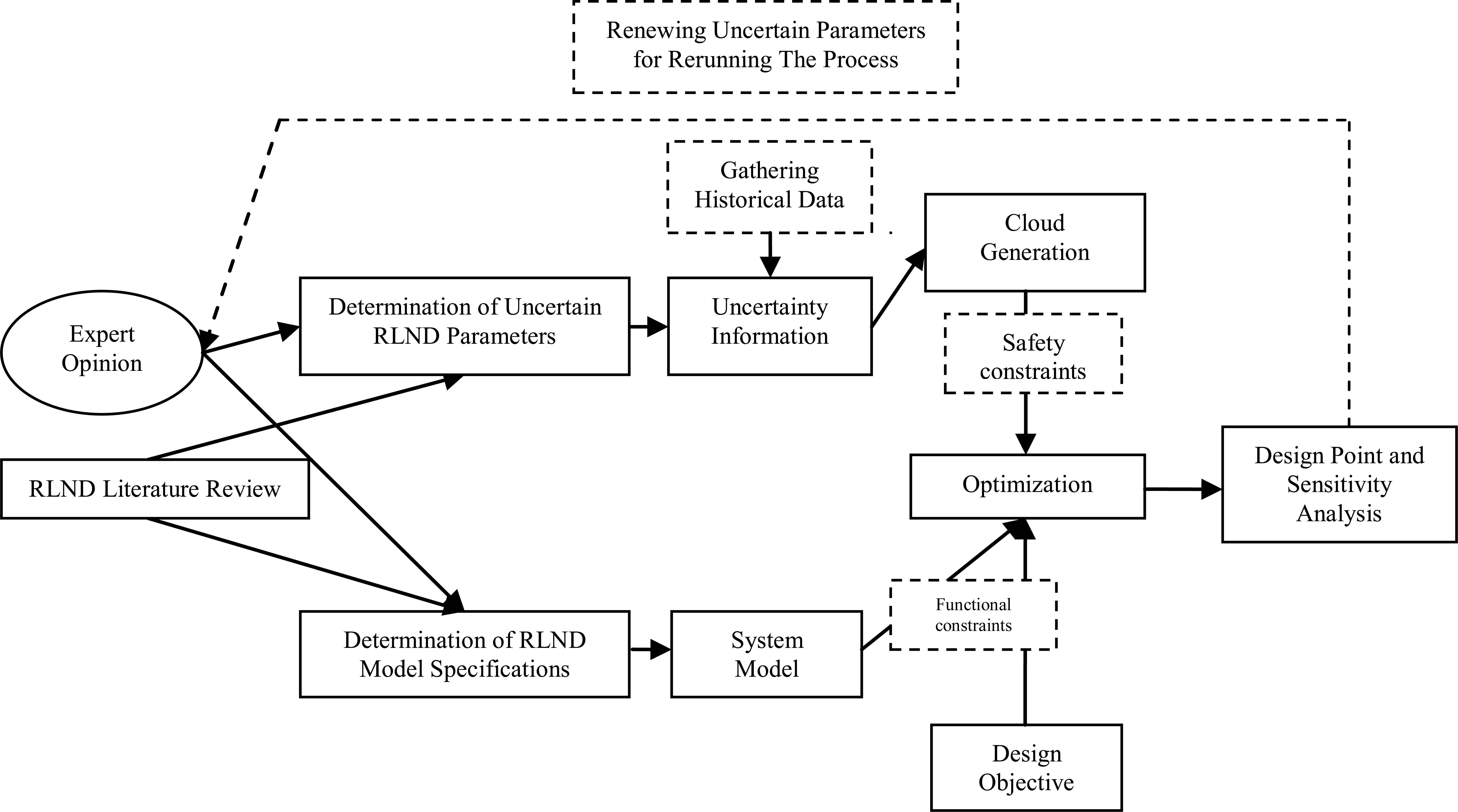
CBDO research framework for multi-period RLND
Assume that ε is the vector of uncertainties. θ is the vector of choice variables. z is the vector consisting of all global input variables (u) and all design variables (v). x is the vector including all output variables. The table constraints assign to each choice a design vector z whose value is the nominal table entry Z(θ) plus its (unknown) error ε with certainty stated by the cloud.
The functional constraints specify the functional relationships in model, which is mostly obtained as a black box. One of the assumptions is the quantity of equations and output variables is the same and they are solvable for x uniquely.
The typical mixed integer CBDO model can be shown as following:
In order to handle the outer level of the Eq. (2) (to find the design choice θ with the minimal worst case objective function value), two different techniques are utilized: (1) a quadratic model (one fits a quadratic model of the objective function and minimizes it); and (2) separable underestimation. The separable underestimation technique has the advantage of the discrete nature of θ and finds a separable underestimation q(θ) for the objective form (See Ref. 40)
- n0=
the dimension of the choice variable
- θi =
the ith coordinate of θ
Let N0 equals the number of function evaluations f1,…,fN0 that have been made in advance for the design choices θ1,…,θN0 . qi(θi) is a constant

General RL network structure
And they are computed by an LP solver. This ensures that many constraints in Eq. (4) will be active. The underestimator q(θ) can then be easily minimized later. The minimizers are utilized as starting points for a limited global search that includes an integer line search for discrete choice variables and multilevel coordinate search for continuous (See Ref. 40).
A typical RL process includes the following steps as illustrated in Fig. 2: First, end of life products are gathered in containers of distributors. Then, returned products are collected in collection centers. Manual inspecting is achieved to separate the units according to their recoverability. The recoverable products are transported to recovery centers, and the remainders are shipped to the disposal centers. The recoverable products are processed at recovery centers and then sold to material suppliers (MS) while the remainder is sent to disposal centers.
The goal of our study is to decide on the best arrangement while minimizing total cost under high uncertainty. In the extant literature, the RL design problems are formulated both as a cost minimization (See Ref. 29) and profit maximization (See Ref. 20). We formulated a multi-period reverse logistics network design problem for an electric and electronic recycling company seeking a cost minimization objective. The company does not expect profit maximization from the reverse logistics operations rather it aims to satisfy the WEEE regulations by a minimum-cost reverse logistics design.
For this initial and pure case, some assumptions are considered to decrease the complex nature of the problem such as: (1) Inventory costs are ignored; (2) There is no capacity constraint on centers; (3) Inspection rates at collection centers and material amount rates obtained at recycling centers are uncertain parameters which are stochastic; (4) Operation costs, opening costs and transportation costs are uncertain parameters which are stochastic.
The reverse logistics network design model will lead to select the best locations and allocations with the aim of minimum cost by considering four multiple periods (p=1,2,…). It is stated that in the first period the decision of opening centers will be made and the allocations of units between centers will change over time.
The formulation of CBDO based multi-period reverse logistics network design model contains three main phases:
- •
Phase 1: Determination of probabilistic uncertain parameters
- •
Phase 2: Determination of parameters, variables and objective function
- •
Phase 3: Structuring the CBDO model
Phase 1: Determination of probabilistic uncertain parameters
Parallel to technological developments and investments made on recovery systems, performance of recovery has increased and it directly affects the inspection rate and the quantity of materials recovered from products. In our model, fluctuating parameters; inspection amount, material amount rates, and operation, opening and transportation costs are considered stochastic. It is assumed that stochastic parameters are normally distributed with a given mean and a standard deviation.
- Llp
denotes percentage of recyclable material amount obtained at collection center l at period p;
- Mmp
denotes percentage of material amount obtained at recycling center m at period p;
- FLlp
denotes opening cost of collection center l at period p;
- FMmp
denotes opening cost of recycling center m at period p;
- CLlp
denotes unit operation cost of collection center l at period p;
- CMmp
denotes unit operation cost of recycling center m at period p;
- KCklp
denotes cost of shipping one unit from collection point k to collection center l at period p;
- LClmp
denotes cost of shipping one unit from collection center l to recovery center m at period p;
- LDldp
denotes cost of shipping one unit from collection center l to disposal center d at period p;
- MDmdp
denotes cost of shipping one unit from recycling center m to disposal center d at period p;
- MSmsp
denotes cost of shipping one unit from recovery center m to material supplier s at period p.
The multi-period reverse logistics problem we model includes a much higher number of uncertain criteria. It is large enough to develop a representative case for dealing with uncertainty by utilizing CBDO.
Phase 2: Determination of parameters, variables and objective function
Seven variables that refer to the connection indicators and choice of opening centers are involved in the model. For each period there are 28 uncertain input variables. In total there are 112 uncertain input variables including 4 periods. The details of the CBDO model are given as the following:
- k ∈ K =
set of collection points
- l ∈ L =
set of collection center locations
- m ∈ M =
set of recycling center locations
- d ∈ D =
set of disposal center locations
- s ∈ S =
set of material supplier locations
- p ∈ P =
set of periods
- Qkp =
return amount at collection point k at period p
- Llp =
percentage of recyclable material amount obtained at collection center l at period p
- Mmp =
percentage of material amount obtained at recycling center m at period p
- FLlp =
annualized fixed costs for opening collection center l at period p
- FMmp =
annualized fixed costs for opening recycling center m at period p
- CLlp =
unit operation cost of collection center l at period p
- CMmp =
unit operation cost of recycling center m at period p
- KCklp =
cost of shipping one unit from collection point k to collection center l at period p
- LClmp =
cost of shipping one unit from collection center l to recovery center m at period p
- LDldp =
cost of shipping one unit from collection center l to disposal center d at period p
- MDmdp =
cost of shipping one unit from recycling center m to disposal center d at period p
- MSmsp =
cost of shipping one unit from recovery center m to material supplier s at period p
- llp =
selection of collection center l and it equals to 1 if collection center l is selected, 0 otherwise at period p
- mmp =
selection of recycling center m and it equals to 1 if recycling center m is selected, 0 otherwise at period p
- klklp =
indicator connecting collection point k and collection center l at period p
- lmlmp =
indicator connecting collection center l and recycling center m at period p
- ldldp =
indicator connecting collection center l and disposal center d at period p
- mdmdp =
indicator connecting recycling center m and disposal center d at period p
- msmsp =
indicator connecting recycling center m and material supplier s at period p
The main goal is to select the best network design option by considering the design objective mcos t which includes cost minimization. mcos t is the sum of cost items given in Eq. (5)–(12).
In the CBDO model, θi is the choice of network design option with the minimum cost. Each choice is specified by 80 main design variables
4.2. Comparison of CBDO using a Numerical RLND Example
In this part, we aim to compare chance constraint programming, stochastic programming approach, fuzzy programming and cloud based design optimization by using an illustrative numerical example. The indices, parameters and variables used at the following formulations are listed below:
- i =
number of potential warehouse locations
- j =
number of markets
- Dj =
annual demand of market j
- Fi =
fixed cost of locating a warehouse at site i
- Cij =
cost of shipping one unit from warehouse i to market j
- P =
probability of stochastic (demand) constraint
- Yi =
1 if warehouse is located at site i, 0 otherwise
- Lij =
1 if allocation from warehouse i to market j is open, 0 otherwise
- Xij =
quantity shipped from warehouse i to market j
The illustrative numerical example solved in this section has one echelon simple network that includes three warehouses and two markets. It is assumed that the demands of two markets are uncertain. The objective is to minimize the total costs. The parameters values for the illustrative numerical example are given at Table 2.
| D1 = normally distributed with mean 80 and st.dev. 20 | C11 =5 $/unit |
| D2 = normally distributed with mean 100 and st.dev. 40 | C12 =10 $/unit |
| F1 =1000 $ | C21 =6 $/unit |
| F2 =1250 $ | C22 =12 $/unit |
| F3 =1500 $ | C31 =8 $/unit C32 =16 $/unit |
Parameters of chance constraint programming
4.2.1. Chance constraint programming
The chance constraint programming model for the RLND problem is:
The constraint probability is assumed to be αi =0.9
Normally distributed demand constraints are:
X11 + X21 + X31 = D1 * L11 + D1 + L21 + D1 * L31
X12 + X22 + X32 = D2 * L12 + D2 + L22 + D2 * L32
Risk adjusted demand constraints are:
X11 + X21 + X31 = D1 * L11 + D1 + L21 + D1 * L31 − 1,282 * 20
X12 + X22 + X32 = D2 * L12 + D2 + L22 + D2 * L32 − 1,282 * 40
The model is run by utilizing GAMS CPLEX solver. The results reveal out that minimum cost is 1759$ and a decision of opening the first warehouse is made.
4.2.2. Two stage stochastic programming
The general location-allocation model is proposed by considering the studies of Ref. 41 and Ref. 42 which are originated from general formulation stated by Ref. 43
The number of scenarios is indexed by s and probability of each scenarios (if probability is same for each scenario, then it is = 1/scenario amount) is represented as qs. Then, the two stage stochastic programming RNLD model is formulated as:
A numerical study is conducted by considering that there are three warehouses and two markets and ten scenarios. The values of the parameters are same as the chance constraint programming model. Additionally, the probability of each scenario is set as 1/10.
The model is run by utilizing GAMS CPLEX solver. The results reveal out that minimum cost is 2494,83 $. The open decision is made for the first warehouse.
4.2.3. Fuzzy programming
According to the study of Ref. 44, uncertain demand can cause uncertain penalty costs for overages and shortages. Similarly, in our case, it is assumed that if the needed demand is not met as it is requested, then penalty cost occurs. The fuzzy programming of a facility location allocation model is given below:
| Ni | n1 = y1 | n2 = y2 | n3 = y3 | n4 =l11 | n5 =l12 | n6 =l21 | n7 =l22 | n8 =l31 | n9 =l32 |
|---|---|---|---|---|---|---|---|---|---|
| Combination Alternatives = Possible Choices | Open warehouse 1 (i1) | Open warehouse 2 (i2) | Open warehouse 3 (i3) | Open linkage (i1 to j1) | Open linkage (i1 to j2) | Open linkage (i2 to j1) | Open linkage (i2 to j2) | Open linkage (i3 to j1) | Open linkage (i3 to j2) |
| N1 = 1 | 1 | 0 | 0 | 1 | 1 | 0 | 0 | 0 | 0 |
| N2 = 2 | 0 | 1 | 0 | 0 | 0 | 1 | 1 | 0 | 0 |
| N3 = 3 | 0 | 0 | 1 | 0 | 0 | 0 | 0 | 1 | 1 |
Input values of CBDO (in comparative example)
For our example, if the demand exceeds the expected demand, then overage penalty cost (0,1 $/unit) is considered. If the demand is under the expected demand, then shortage penalty cost (0,4 $/unit) is considered. And total penalty cost
The model is solved by considering all of these options separately by utilizing GAMS CPLEX solver. That means the model is run for all demand combinations (from the most pessimistic one to the most optimistic one). The optimum result is 2369,5 $ and first warehouse is open.
4.2.4. Cloud based design optimization
CBDO is developed for alternative warehouse selections. In our case θi is the choice of location and its linkages with the minimum cost (that is the total of transportation and facility opening costs). Each choice is specified by 9 main design variables
The graphical user interface (GUI) of CBDO is used in order to declare the elements of the model. First model is declared as GUI needs. Then the uncertainty elicitation is represented. In the following step available information is entered to form the clouds which produce the safety constraints for the optimization. The optimization results are obtained in the last step. In CBDO, optimum result is found as 3389,64 $ in total.
The results that are obtained by solving the problem with the above mentioned four solution approaches are compared at Table 4. Since there was no capacity constraint for the warehouses in the model, one warehouse (first one) is selected in all approaches. As it is expected, the highest cost is obtained by CBDO because CBDO conducts a worst case analysis. The results indicate that results are very sensitive to uncertainty and uncertainty can cause high cost.
| Chance Constraint Programming | Two Stage Stochastic Programming | Fuzzy Programming | CBDO | |
|---|---|---|---|---|
| Objective function value ($) | 1759 | 2494,83 | 2369,5 | 3389,64 |
Comparison of the CBDO results with the results of the other solution approaches
5. Case Study and Computational Results
The CBDO model has been validated through WEEE industry to illustrate its performance. We conducted a case study in Turkey because the situation of WEEE in Turkey is challenging. The environmental regulations have been well accepted and implemented in many developed countries; however, it is still a fairly new process for many developing countries such as Turkey. Regional Environmental Centre (REC) Turkey (2012) forecasted that Turkish manufacturers added 812,000 tons of EEE on the market via approximately 20,000 distributors (2012). This high volume of EEE causes a huge volume of WEEE. Turkey tackles with 539,000 tons of WEEE annually. Average growth per year is 5%; therefore, it is expected that 894,000 tons EEE will be obtained in 2020. According to analysis of REC Turkey, if the Directive goes into force successfully, a total of 116,355 unit points of environmental risks to the ecosystem quality to human health and to energy resources can be decreased. The WEEE Directive implementation will also provide many social benefits such as decreasing the informal sector quantity and job creation (REC 2012).
We take into consideration a recycling facility because recycling centres have an important role in RL networks. They are responsible for taking out legal licenses from ministries and using appropriate technologies and techniques for recycling operations. Unless appropriate technologies and techniques are used, hazards for the environment and health could increase and recycling of wastes could be done mostly by unskilled labor. Moreover, most OEMs operate RL activities by collaborating with recycling firms. It is clear the role of recycling centres is significant for fulfillment of an effective sustainable RL network. Therefore, in this study a case study is conducted with the data of the WEEE collection and recycling facility which operates in İzmit-Turkey.
The selected facility is the first licensed Turkish recycling firm built in 1999. It has the highest market share as a recycling firm in this sector. The common recycled WEEE includes monitors, televisions, information technology (IT) and telecommunication equipment. The facility is in collaboration with municipalities, distributors and OEMs for collection of used or scrapped electrical and electronic equipments. In the network of the recycling firm, there are collection points, collection and recycling centres, and disposal centres and material suppliers.
Strategically, the managers of the selected firm believe that after the environmental regulations go into force, the product return amount will increase in the following periods. Therefore, they need to design their RL network by considering different facts of different periods. It is assumed there are five different actors in the alternative networks: three main collection points (k=1,2,3), two alternative collection centers (l=1,2), two alternative recycling centers (m=1,2), one main disposal center (d=1) and one main material supplier (s=1).
The reverse logistics network design model will lead to select the best locations and allocations with the aim of minimum cost by considering four main periods (one period refers to one year) (p=1,2,3,4). It is stated that in the first period the decision of opening centers will be made and the allocations of units between centers will change over time. The returned amounts are expected to increase over time because of the effects of force environmental regulations and to increase in the consciousness of consumers. The return amounts on collection points for each period (Qkp) is gathered by considering the obligation amounts of WEEE regulation.
For historical data set gathering, we limited the time span to the last two years to prevent the effects of out of date parameters which address the conditions in Turkey before adaptation. Uncertain parameters are analyzed for each month of two years. According to historical data analysis, it is assumed that stochastic parameters are normally distributed with the mean of values and standard deviations are given in Table 5. The values of means and standard deviations are revealed by considering historical data of the last two years.
In CBDO literature, it is stated the CBDO is an effective support tool especially for high dimensional problems. If number of uncertainties in a problem exceeds five, it means the problem has high uncertainty-- in other words, “high dimensionality” (See Ref 40). In our case study, the number of uncertain criteria considered in CBDO equals 112 (is the total of uncertainties given in Table 5). Seven variables that refer to the connection indicators and choice of opening centers are involved in the model. For each period there are 28 uncertain input variables. In total there are 112 uncertain input variables including 4 periods. By entering the values of certain and uncertain parameters, the model is run by using the CBDO graphical user interface (GUI) software which is set up by Ref. 40.
| Period 1 | L11 | L21 | M11 | M21 | FL11 | FL21 | FM11 | FM21 | |||
| Mean | 70 | 70 | 80 | 80 | 2000 | 2400 | 3500 | 3000 | |||
| St.dev. | 35 | 40 | 40 | 50 | 500 | 720 | 1050 | 1500 | |||
| CL11 | CL21 | CM11 | CM21 | KC111 | KC121 | KC211 | KC221 | KC311 | KC321 | ||
| Mean | 2.5 | 3 | 4 | 5 | 3 | 2 | 3 | 3 | 3 | 3 | |
| St.dev. | 0.5 | 1.5 | 2 | 1.5 | 1 | 1.2 | 1.2 | 1.5 | 1.5 | 1.2 | |
| LC111 | LC121 | LC211 | LC221 | LD111 | LD211 | MD111 | MD211 | MS111 | MS211 | ||
| Mean | 3 | 3.5 | 5 | 4 | 2 | 2 | 2.5 | 2.5 | 2 | 2 | |
| St.dev. | 1.5 | 0.7 | 2.5 | 2 | 1 | 1 | 0.5 | 0.5 | 0.4 | 0.4 | |
| Period 2 | L12 | L22 | M12 | M22 | FL12 | FL22 | FM12 | FM22 | |||
| Mean | 75 | 75 | 85 | 85 | 0 | 0 | 0 | 0 | |||
| St.dev. | 35 | 30 | 45 | 42 | - | - | - | - | |||
| CL12 | CL22 | CM12 | CM22 | KC112 | KC122 | KC212 | KC222 | KC312 | KC322 | ||
| Mean | 3 | 3 | 4 | 6 | 2 | 1.8 | 2.5 | 2.5 | 3 | 3 | |
| St.dev. | 0.5 | 1.5 | 2.5 | 2 | 0.5 | 1 | 1 | 1.5 | 1 | 1.5 | |
| LC112 | LC122 | LC212 | LC222 | LD112 | LD212 | MD112 | MD212 | MS112 | MS212 | ||
| Mean | 4.5 | 3.8 | 5 | 4 | 2 | 2.5 | 3 | 2.5 | 2.5 | 2 | |
| St.dev. | 1.5 | 2 | 2 | 1.5 | 0.5 | 1.2 | 1.5 | 1 | 1 | 1 | |
| Period 3 | L13 | L23 | M13 | M23 | FL13 | FL23 | FM13 | FM23 | |||
| Mean | 85 | 85 | 90 | 90 | 0 | 0 | 0 | 0 | |||
| St.dev. | 20 | 20 | 30 | 30 | - | - | - | - | |||
| CL13 | CL23 | CM13 | CM23 | KC113 | KC123 | KC213 | KC223 | KC313 | KC323 | ||
| Mean | 3.5 | 3.2 | 4.4 | 6 | 5 | 2 | 3 | 3 | 3.2 | 3.5 | |
| St.dev. | 1 | 1.5 | 2.5 | 3 | 1 | 1 | 1.5 | 1.5 | 1.5 | 1.5 | |
| LC113 | LC123 | LC213 | LC223 | LD113 | LD213 | MD113 | MD213 | MS113 | MS213 | ||
| Mean | 6 | 4 | 5.2 | 4.4 | 3 | 2.5 | 4 | 3 | 3 | 2.4 | |
| St.dev. | 1.8 | 2 | 2 | 1.5 | 1.5 | 1 | 1.5 | 1.5 | 1.5 | 1 | |
| Period 4 | L14 | L24 | M14 | M24 | FL14 | FL24 | FM14 | FM24 | |||
| Mean | 88 | 88 | 92 | 92 | 0 | 0 | 0 | 0 | |||
| St.dev. | 20 | 20 | 30 | 30 | - | - | - | - | |||
| CL14 | CL24 | CM14 | CM24 | KC114 | KC124 | KC214 | KC224 | KC314 | KC324 | ||
| Mean | 3.5 | 3.5 | 4.5 | 6 | 3.5 | 2.5 | 4 | 4 | 3.5 | 3.5 | |
| St.dev. | 1.5 | 1.5 | 2.5 | 3 | 1.5 | 1 | 1.5 | 1.5 | 1.5 | 1.5 | |
| LC114 | LC124 | LC214 | LC224 | LD114 | LD214 | MD114 | MD214 | MS114 | MS214 | ||
| Mean | 4 | 4 | 5.5 | 4.4 | 3 | 3 | 4 | 3.5 | 3.5 | 2.5 | |
| St.dev. | 2 | 2 | 2 | 2 | 1 | 1.5 | 2 | 1.5 | 1.5 | 1 | |
Mean and standard deviation values of normally distributed stochastic parameters of all periods
In our case, there are four network design alternatives (possible choices) therefore, Ni = 4. The network design alternatives and linkages between centers can be seen in Fig. 3.
In the model, θi is the choice of network design option with the minimum cost. Each choice is specified by 80 main design variables
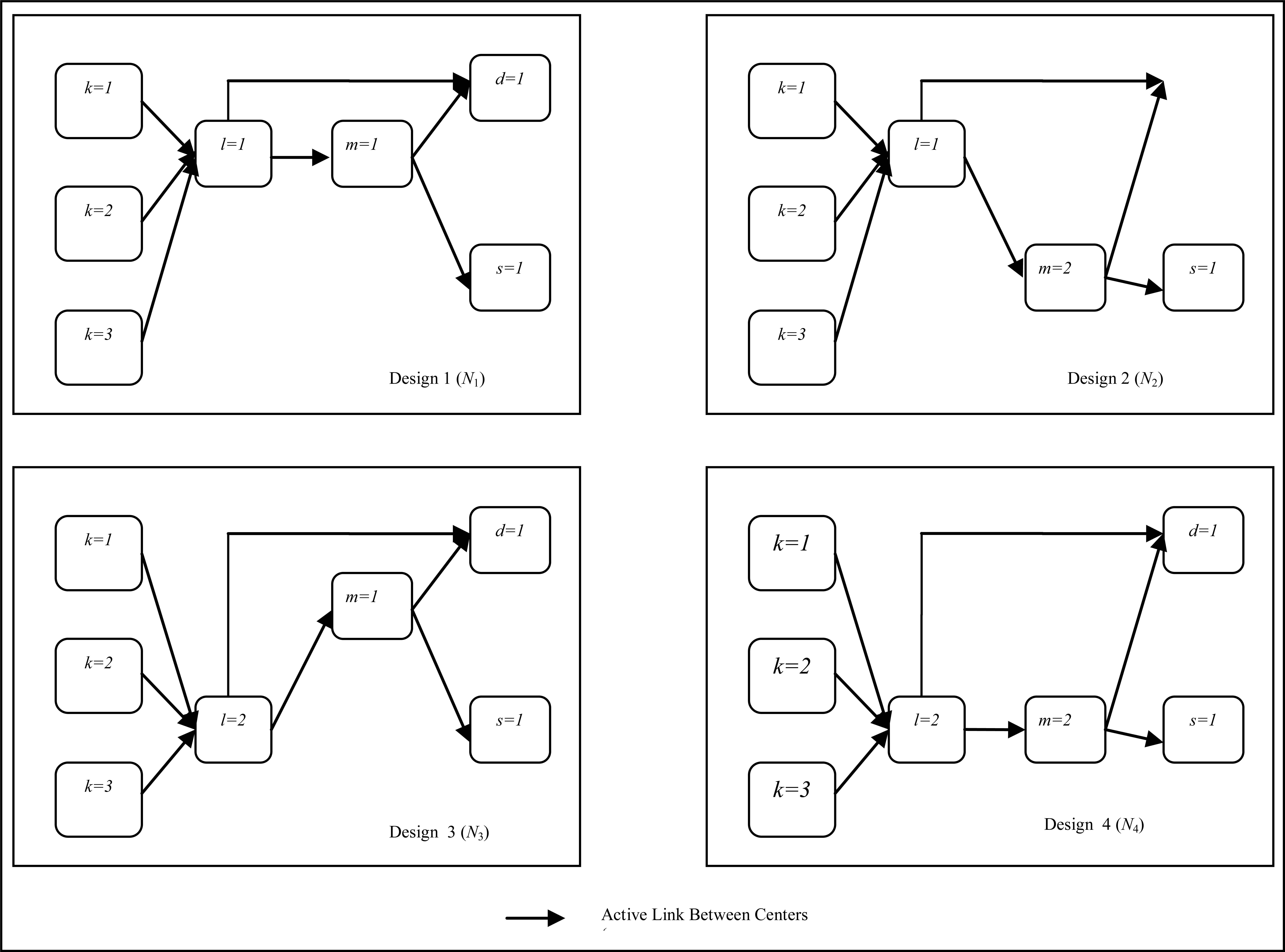
Design options.
That means products collected in all containers are sent to the first collection center. Then, the products which are found as unrecoverable are shipped from first collection center to the disposal center (ld111 = 1). The remainder are passed through recycling operations in the first recycling center (m11 = 1) in order to obtain raw materials. The recovered materials are shipped from the recycling center to the supplier (ms111 = 1) and unrecoverable materials are sent to the disposal center (md111 = 1). These input values are the table constraints of CBDO and all values of network design option can be seen in Table 6.
Specifications of the model are determined as CBDO’s specific necessities by clarifying objective function, input (global and design) variables, fixed data, and distributions of uncertain data. Confidence level is selected as 0.95 for cloud generation and as 0.998 for sample generation. The generated sample size of CBDO is 1,000 for the cloud generation stage. The transformation function is chosen as logarithmic. The iteration for weight computation is selected as 3,000.The number of starting points is randomly defined by the software. The results are confirmed two times in order to check the accuracy. The principle of optimization depends on local search.
The model is coded in CBDO GUI and run by using a computer which has an Intel Core i5 CPU with 2.26 GHz, 4 GB RAM and a 64 bit operating system. The CPU time equals 3.61 seconds. In order to compare CPU time performance of the model, the first echelon of network is modeled by two alternative programming: two stage stochastic programming and fuzzy programming. In two-stage stochastic programming, the decisions set can be categorized into two groups: (1) First stage decisions which include decisions made before the experiment; and (2) Second stage decisions which include decisions made after experiment. In a traditional two stage stochastic facility location, the allocation model includes the first stage decisions as opening the facility and second stage stochastic programming as allocation of units between facilities (See Ref. 43). The proposed stochastic model is run by utilizing GAMS CPLEX solver and its CPU time is found as 6.9 seconds. Furthermore, a fuzzy programming is developed by considering the model of Ref. 44. In our case, it is assumed that if the needed demand is not met as it is requested, then the penalty cost occurs. The model is solved by considering all demand combinations (from the most pessimistic one to the most optimistic one) separately by utilizing GAMS CPLEX solver. Its CPU time equals to 6.75 seconds. Compared to stochastic and fuzzy programming, CBDO which intervenes between fuzzy set theory and stochastic distributions offers the best CPU time. Under high uncertainty, it may be impossible to succeed the real quality of approximate solutions. Because of the hardness of dealing with a many uncertain parameters simultenously, heuristic optimization techniques are prefered in many cases. In this case, because CBDO provides heuristic solution that includes iterative process, generation of results becomes faster compared to stochastic and fuzzy programming.
| n1 | n2 | n3 | n4 | n5 | n6 | n7 | n8 | n9 | n10 | n11 | n12 | n13 | n14 | n15 | n16 | n17 | n18 | n19 | n20 | |
| kl111 | kl121 | kl211 | kl221 | kl311 | kl321 | l11 | l21 | lm111 | lm121 | lm211 | lm221 | ld111 | ld211 | m11 | m21 | ms111 | ms211 | md111 | md211 | |
| N1 | 1 | 0 | 1 | 0 | 1 | 0 | 1 | 0 | 1 | 0 | 0 | 0 | 1 | 0 | 1 | 0 | 1 | 0 | 1 | 0 |
| N2 | 1 | 0 | 1 | 0 | 1 | 0 | 1 | 0 | 0 | 1 | 0 | 0 | 1 | 0 | 0 | 1 | 0 | 1 | 0 | 1 |
| N3 | 0 | 1 | 0 | 1 | 0 | 1 | 0 | 1 | 0 | 0 | 1 | 0 | 0 | 1 | 1 | 0 | 1 | 0 | 1 | 0 |
| N4 | 0 | 1 | 0 | 1 | 0 | 1 | 0 | 1 | 0 | 0 | 0 | 1 | 0 | 1 | 0 | 1 | 0 | 1 | 0 | 1 |
| n21 | n22 | n23 | n24 | n25 | n26 | n27 | n28 | n29 | n30 | n31 | n32 | n33 | n34 | n35 | n36 | n37 | n38 | n39 | n40 | |
| kl112 | kl122 | kl212 | kl222 | kl312 | kl322 | l12 | l22 | lm112 | lm122 | lm212 | lm222 | ld112 | ld212 | m12 | m22 | ms112 | ms212 | md112 | md212 | |
| N1 | 1 | 0 | 1 | 0 | 1 | 0 | 1 | 0 | 1 | 0 | 0 | 0 | 1 | 0 | 1 | 0 | 1 | 0 | 1 | 0 |
| N2 | 1 | 0 | 1 | 0 | 1 | 0 | 1 | 0 | 0 | 1 | 0 | 0 | 1 | 0 | 0 | 1 | 0 | 1 | 0 | 1 |
| N3 | 0 | 1 | 0 | 1 | 0 | 1 | 0 | 1 | 0 | 0 | 1 | 0 | 0 | 1 | 1 | 0 | 1 | 0 | 1 | 0 |
| N4 | 0 | 1 | 0 | 1 | 0 | 1 | 0 | 1 | 0 | 0 | 0 | 1 | 0 | 1 | 0 | 1 | 0 | 1 | 0 | 1 |
| n41 | n42 | n43 | n44 | n45 | n46 | n47 | n48 | n49 | n50 | n51 | n52 | n53 | n54 | n55 | n56 | n57 | n58 | n59 | n60 | |
| kl113 | kl123 | kl213 | kl223 | kl313 | kl323 | l13 | l23 | lm113 | lm123 | lm213 | lm223 | ld113 | ld213 | m13 | m23 | ms113 | ms213 | md113 | md213 | |
| N1 | 1 | 0 | 1 | 0 | 1 | 0 | 1 | 0 | 1 | 0 | 0 | 0 | 1 | 0 | 1 | 0 | 1 | 0 | 1 | 0 |
| N2 | 1 | 0 | 1 | 0 | 1 | 0 | 1 | 0 | 0 | 1 | 0 | 0 | 1 | 0 | 0 | 1 | 0 | 1 | 0 | 1 |
| N3 | 0 | 1 | 0 | 1 | 0 | 1 | 0 | 1 | 0 | 0 | 1 | 0 | 0 | 1 | 1 | 0 | 1 | 0 | 1 | 0 |
| N4 | 0 | 1 | 0 | 1 | 0 | 1 | 0 | 1 | 0 | 0 | 0 | 1 | 0 | 1 | 0 | 1 | 0 | 1 | 0 | 1 |
| n61 | n62 | n63 | n64 | n65 | n66 | n67 | n68 | n69 | n70 | n71 | n72 | n73 | n74 | n75 | n76 | n77 | n78 | n79 | n80 | |
| kl114 | kl124 | kl214 | kl224 | kl314 | kl324 | l14 | l24 | lm114 | lm124 | lm214 | lm224 | ld114 | ld214 | m14 | m24 | ms114 | ms214 | md114 | md214 | |
| N1 | 1 | 0 | 1 | 0 | 1 | 0 | 1 | 0 | 1 | 0 | 0 | 0 | 1 | 0 | 1 | 0 | 1 | 0 | 1 | 0 |
| N2 | 1 | 0 | 1 | 0 | 1 | 0 | 1 | 0 | 0 | 1 | 0 | 0 | 1 | 0 | 0 | 1 | 0 | 1 | 0 | 1 |
| N3 | 0 | 1 | 0 | 1 | 0 | 1 | 0 | 1 | 0 | 0 | 1 | 0 | 0 | 1 | 1 | 0 | 1 | 0 | 1 | 0 |
| N4 | 0 | 1 | 0 | 1 | 0 | 1 | 0 | 1 | 0 | 0 | 0 | 1 | 0 | 1 | 0 | 1 | 0 | 1 | 0 | 1 |
Input values of CBDO model
Furthermore, CBDO has another advantage that enables decision makers have confirmation on results, as a testing procedure. The results of the case are confirmed twice within GUI and the total cost is found as 135,618,000 monetary units.
The results indicate the 3rd network design where the second collection center (l2 = 1) and first recovery center (m1 = 1) are open should be selected.
It is required to serve product returns from all collection points to a second collection center and sending manually inspected products from a second collection center to the first recycling center. The remainder of the products is sent to the disposal center. After recycling is completed in the first recycling center, materials are shipped to material supplier and the rest of them are sent to the disposal center. It is a two times tested result and makes decision makers handle uncertainties in a reliable manner although there is a lack of information. Under highly uncertain conditions of WEEE recycling process, for managers it is more helpful to consider worst case based results for safeguarding the firm against unsteadiness caused due to imprecise data.
Finally, a sensitivity analysis is conducted to explore the effect of changing in standard deviation (SD).With the goal of understanding how total cost and opening decisions will change if the fluctuations vary because of some unexpected situations. Therefore, the model is run for increasing and decreasing SDs. Four different scenarios are taken into consideration:
- (1)
standard deviation values are equal to mean value;
- (2)
standard deviation values are increased by 75 percentage points;
- (3)
standard deviation values are decreased by 50 percentage points; and
- (4)
standard deviation values are decreased by 90 percentage points.
For Scenario 1, it is believed the total cost will increase to 1,306,264,541. For Scenarios 2, 3 and 4, the total costs are 302,416,836; 46,906,395 and 10,558,653 monetary units, respectively. High volume increase in total cost indicates that higher fluctuations in parameters cause more risky and costly results. It is evident that the total cost converges with decreasing standard deviations as seen in Fig. 4.
Except for Scenario 1, all scenarios result with the opening second collection center (l2 = 1) and first recovery center (m1 = 1). However, the results of Scenario 1 address that opening via the first collection center (l1 = 1) and the first recovery center (m1 = 1) is preferable. It is seen that fluctuations resulting in a high level of uncertainty have a direct impact on opening decisions. Therefore, the trends in the sector should be reviewed in detail by managers and if there is high potential to meet with risky situations in the future, the effectiveness of collection centers should be criticized again.
The case study shows that consideration of uncertainty and changing the amounts of the product-returns would have direct impact on the results. Decision makers should not ignore the imprecise parameters of the RLND problem. The results obtained from our CBDO model show that the optimal design point is sensitive to whether the uncertainty is considered in the model or not. Experts must track product return trends and have optimistic foresight, expected and pessimistic returns in various periods. CBDO application contributes to the literature by revealing the necessity to consider uncertainties as one of vital responsibility for decision makers in RLND problems.
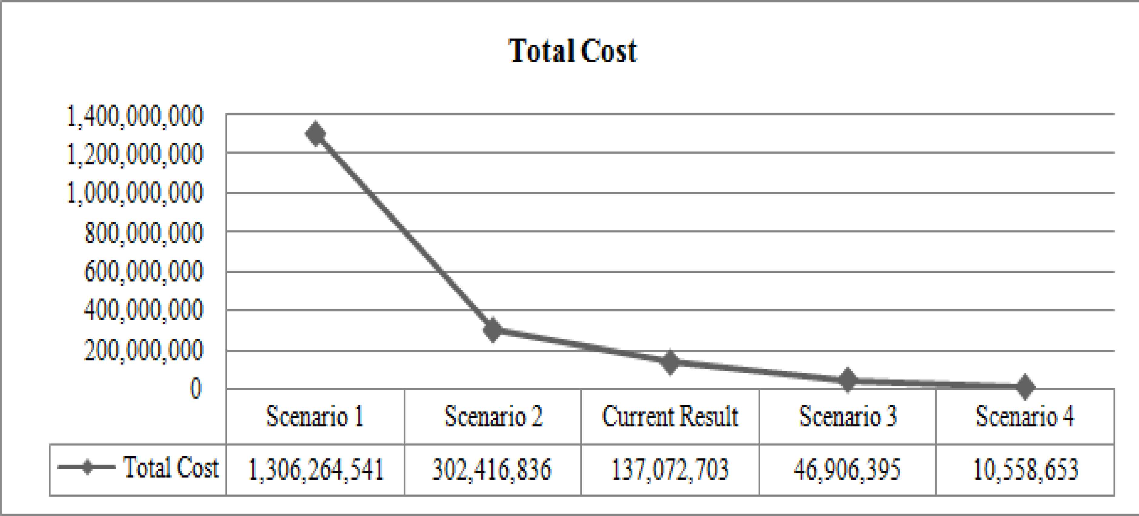
Sensitivity analysis results
6. Conclusion
In recent years, RL has become increasingly important in many sectors. RLND, which is one of important strategic decisions in RL study, contains uncertain structure and has potential to increase the complexity of decision making process on facility location allocation problems. High uncertainty that is not considered in decision-making can cause high costs and wasted time because it will lead to wrong planning. Therefore, it becomes inevitable to benefit from an effective decision making tool in order to challenge high uncertainty. Under these circumstances, this study proposes a general, multi-echelon, multi-period, single product, cost minimization RLND model. A new notion titled CBDO is in order to handle high quantity of certain and uncertain factors simultaneously. It identifies best solution within worst case scenario. Only few approaches such as simulation, fuzzy theory and stochastic programming can tackle the cases including high level of incomplete information. However they are able to deal with low dimensions and need high computational effort. CBDO can handle high dimensionality and can help the decision makers to have foresight about the riskiest conditions and take necessary action on time.
To the best of our knowledge, this study is the first in which the CBDO model is used for the decision of a logistics network design based industrial problem. CBDO, which provides a baseline for high number of various uncertainty assessments, can be used as guidelines for RLND problems. A motivating study is conducted to validate performance of the proposed model. The results show this system can help managers to make decisions on facility selection. Directions for future studies may include: (1) new issues that can also be added into the methodology, such as lot sizing, vehicle routing, and inventory management; (2) considering more uncertain parameters; and (3) integrating fuzziness to tackle epistemic uncertainties within CBDO.
Acknowledgment
This research has been conducted in partial support of the Istanbul Technical University Scientific Research Projects (ITU-BAP) Grant #38319. The authors are thankful to ITU-BAP for this support.
References
Cite this article
TY  - JOUR
AU  - Gül T. Temur
AU  - Seda Yanık
PY  - 2017
DA  - 2017/08/21
TI  - A Novel Approach for Multi-Period Reverse Logistics Network Design under High Uncertainty
JO  - International Journal of Computational Intelligence Systems
SP  - 1168
EP  - 1185
VL  - 10
IS  - 1
SN  - 1875-6883
UR  - https://doi.org/10.2991/ijcis.2017.10.1.77
DO  - 10.2991/ijcis.2017.10.1.77
ID  - Temur2017
ER  -