
Numerical Solution of Fuzzy Differential Equations with Z-numbers Using Bernstein Neural Networks
- DOI
- 10.2991/ijcis.10.1.81How to use a DOI?
- Keywords
- Fuzzy differential equations; Bernstein neural networks; Z- numbers; Uncertain nonlinear systems
- Abstract
The uncertain nonlinear systems can be modeled with fuzzy equations or fuzzy differential equations (FDEs) by incorporating the fuzzy set theory. The solutions of them are applied to analyze many engineering problems. However, it is very difficult to obtain solutions of FDEs.
In this paper, the solutions of FDEs are approximated by two types of Bernstein neural networks. Here, the uncertainties are in the sense of Z-numbers. Initially the FDE is transformed into four ordinary differential equations (ODEs) with Hukuhara differentiability. Then neural models are constructed with the structure of ODEs. With modified back propagation method for Z-number variables, the neural networks are trained. The theory analysis and simulation results show that these new models, Bernstein neural networks, are effective to estimate the solutions of FDEs based on Z-numbers.
- Copyright
- © 2017, the Authors. Published by Atlantis Press.
- Open Access
- This is an open access article under the CC BY-NC license (http://creativecommons.org/licences/by-nc/4.0/).
1. Introduction
Since the uncertainty in parameters can be transformed into fuzzy set theory [1] , fuzzy set and fuzzy system theory are good tools to deal with uncertainty systems. Fuzzy models are applied for a large class of uncertainty nonlinear systems, for example Takagi-Sugeno fuzzy model [2] . When the parameter of an equation are changeable in the manner of fuzzy set, this equation becomes a fuzzy equation [3] . When the parameters or the states of the differential equations are uncertain, they can be modeled with FDE.
Many FDEs use fuzzy numbers as the coefficients of the differential equations to describe the uncertainties[4] . The applications of these FDEs are connection with nonlinear modeling and control [5–8]. Another type of FED uses fuzzy variables to express the uncertainties. The study on the solutions of FDEs are applied into chaotic analysis, quantum system and many engineering problems, such as civil engineering and modeling actuators. The basic idea of fuzzy derivative was first introduced in [9] . Then it is extended in [10] . The linear first-order equation is the most generalized FDE. By generalizing the differentiability, [11] gives an analytical solution. In [12] , the first order FDE with periodic boundary conditions is analyzed. Then higher order linear FDE are studied. In [13] , the analytical solutions of second order FDE are obtained. The analytical solutions of third order linear FDE are found in [14] .
Too much complexity is involved in solving nonlinear FDE. By interval-valued method, [15] examines the basis solutions nonlinear FDEs with generalized differentiability. [16] uses periodic boundary and Hukuhara differentiability to the impulsive FDE. [17] suggests some suitable criterion to fuzzify the crisp solutions. [18] uses two-point fuzzy boundary value for FDE. However, all of above analytical methods for the solutions of FDEs are very difficult, especially for nonlinear FDEs.
Numerical solutions of FDEs have been discussed by many scientists recently. The numerical solutions of first-order FDE is proposed in [19] with an iterative technique. [20] uses Laplace transform for second-order FDE. By extending classical fuzzy set theory, [21] obtains numerical solution of an FDE. The predictor-corrector approach is applied in [22] . Euler numerical technique is used in [23] to solve FDE. Some other numerical techniques, such as Nystrom approach [24] , Taylor method [25] and Runge-Kutta approach [26] can also be applied to solve FDEs. However the approximation accuracy of these numerical calculations are normally less.
The solution of FDE is uniformly continuous and inside compact sets [27] . Neural networks can give a good estimation for the solutions of FDEs. [28] shows that the solution of ODE can be approximated by neural network. [29] discusses differences between the exact solution and approximation solutions of ODEs. [30] applies dynamics neural networks to approximate first-order ODE. There are few works on FDE. [31] suggests a static neural network to solve FDE. Since the structure of the neural network is not suitable for FDE, the approximation accuracy is poor.
The decisions are carried out based on knowledge. In order to make the decision fruitful, the knowledge acquired must be credible. Z-numbers connect to the reliability of knowledge [32] . Many fields related to the analysis of the decisions are actually use the ideas of Z-numbers. Z -numbers are much less complex to calculate compared with nonlinear system modeling methods. The Z-number is abundantly adequate number compared with the fuzzy number. Although Z-numbers are implemented in many literatures, from theoretical point of view this approach is not certified completely.
The Z-number is a novel idea that is subjected to a higher potential to illustrate the information of the human being and to use in information processing [32] . Z-numbers can be regarded as to answer questions and carry out the decisions [33] . There are few structure based on the theoretical concept of Z-numbers [34] . [35] proposes a theorem to transfer the Z-numbers to the usual fuzzy sets.
In this paper, a new model named Bernstein neural network is used, which has good properties of Bernstein polynomial for FDE based on Z-number. The Bernstein polynomial has good uniform approximation ability for continuous functions [36] . Also it has innumerable drawing properties, homogeneous shape-sustaining approximation, bona fide estimation and low boundary bias. A very important property of the Bernstein polynomial is that it generates a smooth estimation for equal distance knots [37] . This property is suitable for FDE approximation. For more details regarding Bernstein neural networks, refer to [38, 39].
Two types of neural networks are used namely static and dynamic models, to approximate the solutions of FDEs based on z -numbers. These numerical methods use generalized differentiability of FDEs. The solutions of FDE is substituted into four ODEs. Then the corresponding Bernstein neural networks are applied. Finally, some real examples are used to show the effectiveness of the proposed approximation methods with the Bernstein neural networks.
2. Fuzzy differential equation for uncertain nonlinear system modeling
Consider the following controlled unknown nonlinear system
In this paper, the following differential equation (FDE) is used to model the uncertain nonlinear system (1) ,
In order to use FDE based on Z- numbers, initially some concepts of fuzzy variables and Z-numbers.
Definition 1
(fuzzy variable) If x is:
- 1)
normal, there exists ζ0 ∈ R in such a manner x(ζ0) = 1,
- 2)
convex, x(λζ + (1 – λ)ζ) ≥ min{x(ζ), x(ξ)}, ∀ ζ, ξ ∈ R, ∀ λ ∈ [0,1],
- 3)
upper semi-continuous on R, x(ζ) ≤ x(ζ0) + ε, ∀ ζ∈ N(ζ0), ∀ζ0 ∈ R, ∀ ε > 0, N(ζ0) is a neighborhood,
- 4)
x+ = {ζ∈ ℝ, x(ζ) ∈ E|ℝ → [0,1]} is compact, then x is a fuzzy variable.
The fuzzy variable x can be also represented as [40]
Definition 2
(Z- number) A Z-number has two components Z = [x(ζ), p]. The primary component x(ζ) is termed as a restriction on a real-valued uncertain variable ζ. The secondary component p is a measure of reliability of x. p can be reliability, strength of belief, probability or possibility. When x(ζ) is a fuzzy number and p is the probability distribution of ζ, the Z-number is defined as Z+-number. When both x(ζ) and p are fuzzy numbers, the Z-number is defined as Z− -number.
The Z+ -number carries more information than the Z− -number. In this paper, the definition of Z+ -number is used, i.e., Z = [x, p] x is a fuzzy number and p is a probability distribution.
We use so called membership functions to express the fuzzy number. The most popular membership functions are the triangular function
Definition 3
(α - level of fuzzy number) The fuzzy number x in association to the α -level is illustrated as
Therefore [x]0 = x+ = {ζ∈ R, x(ζ) > 0}. Since α ∈ [0,1], [x]α is a bounded mentioned as
Definition 4
(α - level of Z-numbers) The α -level of the Z-number Z = (x, P) is demonstrated as
Similar with the fuzzy numbers [5] , the Z-numbers are also incorporated with three primary operations: ⊕, ⊝and ⊙. These operations are exhibited by: sum, subtract, multiply, and division. The operations in this paper are different definitions with [1] . The α-level of Z-numbers is applied to simplify the operations.
Let us consider Z1 = (x1, p1) and Z2 = (x2, p2) be two discrete Z-numbers illustrating the uncertain variables ζ1 and ζ2,
The operations for the fuzzy numbers are defined as [5]
The above definitions satisfy the Hukuhara difference [41] ,
Also the above definitions satisfy the generalized Hukuhara difference [42]
If x is a triangular function, the absolute value of the Z-number Z = (x, p) is
Definition 5
(α-level of Z-number valued function) Let
With the definition of Generalized Hukuhara difference, the gH-derivative of F at x0 is expressed as
If we apply the α – level (10) to f(t, x) in (2), then we obtain two Z-number valued functions:
The fuzzy differential equation (2) can be equivalent to the following four ODE
In this paper, the FDE (2) is used to model the uncertain nonlinear system (1), such that the output of the plant x can follow the plant output x1,
This modeling object can be considered as: finding
In fact, the nonlinear system can be modeled by the neural network directly. However, this data-driven black box identification method does not use the model information. While the FDE use the model information of the nonlinear system, such as the brief form of the differential equation.
The following theorems give theory support for nonlinear system modeling via FDEs based on Z-numbers.
Theorem 1
If the Z-number function f and its derivative
Proof.
We utilize Picard’s iteration technique [45] to develop a sequence of Z-number functions φn(t) as
Because
In order to validate that x is continuous, it is necessary to show that for any given ε > 0 there exists δ > 0 in such a manner that |t2 − t1|< δ implies |φ(t2) – φ(t1)|<ε. At par with the notation convenience, we suppose that t1 < t2. It follows that
Now we demonstrate that limn→∞ φn(t) is continuous.
Since
Theorem 2
Assume the following FDE based on Z-numbers
Proof.
If x is a Z-number solution of (21) and
As f0 ∈ Jab(a), the last inequality with β (a) = 0 yields β(t) ≤ 0 and
3. Solving fuzzy differential equation with neural networks
In general, it is difficult to solve the four equations (17) or (2). In this paper, a special neural network named Bernstein neural network is used to approximate the solutions of the FDE (2).
The Bernstein neural network use the following Bernstein polynomial,
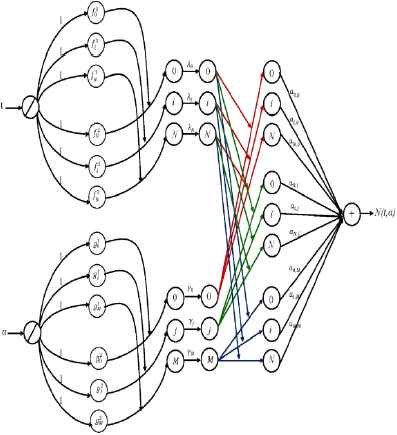
This two variable polynomial can be regarded as a neural network, which has two inputs x1i and x2j and one output y,
Because the Bernstein neural network (27) has similar forms as (17), the Bernstein neural network (27) is used to approximate the solutions of four ODEs in (17), see Figure 1.

Nonlinear system modeling with fuzzy differential equation
If x1 and x2 in (26) are defined as: x1 is time interval t, x2 is the α -level, the solution of (2) in the form of the Bernstein neural network is
So the derivative of (27) is
- •
input unit:
- •
the first hidden units:
- •
the second hidden units:
- •
the third hidden units:
- •
the forth hidden units:
- •
output unit:
where
Static Bernstein neural network
The training errors between (29) and (17) are defined as
The momentum terms, γ∆Wi,j(k−1) and
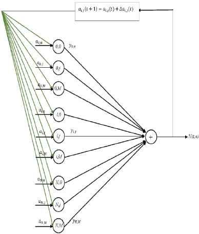
Dynamic Bernstein neural network
The training algorithm is similar as (31), only the training errors are changed as
4. Applications
In this section, several real applications are used to show how to use the Bernstein neural networks to approximate the solutions of the FDEs. These examples can be expressed by FDEs.
Example 1
The vibration mass system shown in Figure 4 can be modeled by the ODE

Vibration mass
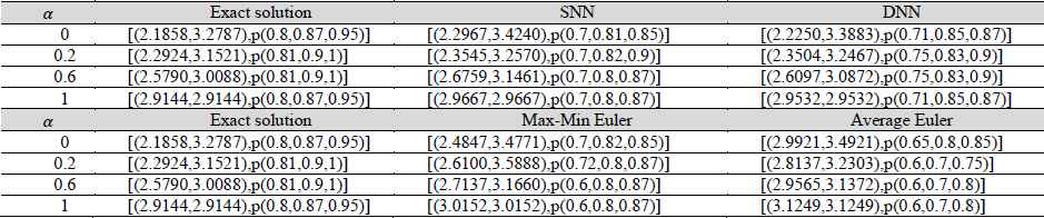
Solutions of different methods based on Z-numbers.
| SNN | DNN | Max-Min Euler | Average Euler | |
|---|---|---|---|---|
| 0 | [(0.0684,0.1251),p(0.7,0.8,0.85)] | [(0.0231,0.0671),p(0.7,0.85,0.87)] | [(0.1064,0.1596),p(0.7,0.8,0.85)] | [[(0.2404,0.5138),p(0.6,0.8,0.85)] |
| 0.2 | [(0.0735,0.1192),p(0.7,0.8,0.9)] | [(0.0266,0.0675),p(0.75,0.8,0.9)] | [(0.1127,0.1551),p(0.7,0.8,0.87)] | [(0.1588,0.4286),p(0.7,0.8,0.85)] |
| 0.6 | [(0.0855,0.1095),p(0.8,0.87,0.95)] | [(0.0339,0.0689),p(0.8,0.9,1)] | [(0.1253,0.1462),p(0.7,0.85,0.9)] | [(0.0082,0.2798),p(0.7,0.81,0.9)] |
| 0.8 | [(0.0833,0.0939),p(0.8,0.91,1)] | [(0.0345,0.0526),p(0.8,0.94,1)] | [(0.1247,0.1345),p(0.8,0.9,1)] | [(0.0628,0.2009),p(0.75,0.9,1)] |
| 1 | [(0.1029,0.1029),p(0.7,0.8,0.9)] | [(0.0572,0.0572),p(0.8,0.85,0.95)] | [(0.1410,0.1410),p(0.7,0.8,0.87)] | [(0.1410,0.1410),p(0.7,0.8,0.87)] |
Approximation errors based on Z-numbers

Comparison plots of SNN, DNN, Max-Min Euler, Average Euler and the exact solution based on Z -numbers
The following relation is used to transfer the Z-numbers to fuzzy numbers,
| α | Exact solution | SNN | DNN | Max-Min Euler | Average Euler |
|---|---|---|---|---|---|
| 0 | [2.0387,3.0581] | [1.9703,3.0043] | [1.9901,3.0305] | [1.9453,2.5980] | [2.2441,2.6191] |
| 0.1 | [2.1067,3.0241] | [2.0302,2.9415] | [2.0591,2.9752] | [2.0102,2.8855] | [2.2791,2.6166] |
| 0.2 | [2.1746,2.9901] | [2.1059,2.9131] | [2.1283,2.9399] | [2.0750,2.8531] | [2.3140,2.6140] |
| 0.3 | [2.2426,2.9561] | [2.1618,2.8707] | [2.1901,2.8931] | [2.1398,2.8207] | [2.3490,2.6115] |
| 0.4 | [2.3105,2.9222] | [2.2307,2.8453] | [2.2601,2.8799] | [2.2047,2.7883] | [2.3840,2.6090] |
| 0.5 | [2.3785,2.8882] | [2.2984,2.8088] | [2.3288,2.8337] | [2.2695,2.7559] | [2.4189,2.6064] |
| 0.6 | [2.4465,2.8542] | [2.3631,2.7784] | [2.3904,2.7955] | [2.3344,2.7234] | [2.4539,2.6039] |
| 0.7 | [2.5144,2.8202] | [2.4292,2.7449] | [2.4555,2.7691] | [2.3992,2.6910] | [2.4888,2.6013] |
| 0.8 | [2.5824,2.7862] | [2.4895,2.7067] | [2.5101,2.7302] | [2.4641,2.6586] | [2.5238,2.5988] |
| 0.9 | [2.6503,2.7523] | [2.5564,2.6769] | [2.5821,2.7001] | [2.5289,2.6262] | [2.5588,2.5963] |
| 1 | [2.7183,2.7183] | [2.6199,2.6399] | [2.6414,2.6614] | [2.5937,2.5937] | [2.5937,2.5937] |
Solutions of different methods based on fuzzy numbers
The Z-numbers increase degree of reliability of the information. The crucial factor is that incorporated information is not only the most generalized representation of information uncomplicated real world but also incorporated with greater narrative power extracted from human cognition perspective compared with fuzzy number. The comparison between the Z-number Z = [(2.1858, 3.2787), p(0.8, 0.87, 0.95)] and fuzzy number [2.0387, 3.0581] is shown in Figure 6. It can be seen that the Z-number incorporates with various information and the solution of the Z-number is more accurate. The membership function for the restriction in the Z-number is μAz = [2.1858,3.2787]. It can be in probability form.
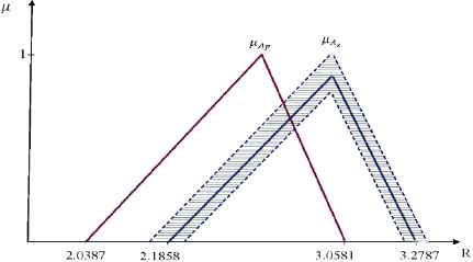
Z-number and fuzzy number
Example 2
The heat treatment system in welding can be modeled as [49]:
| α | SNN | DNN |
|---|---|---|
| 0 | [(0.0582,0.0859),p(0.7,0.8,0.85)] | [(0.0250,0.0425),p(0.7,0.82,0.9)] |
| 0.1 | [(0.0449,0.0696),p(0.7,0.8,0.9)] | [(0.0224,0.0399),p(0.75,0.82,0.9)] |
| 0.2 | [(0.0419,0.0619),p(0.8,0.92,1)] | [(0.0207,0.0394),p(0.8,0.94,1)] |
| 0.3 | [(0.0250,0.0348),p(0.7,0.81,0.9)] | [(0.0226,0.0344),p(0.8,0.85,0.96)] |
| 0.4 | [(0.0487,0.0689),p(0.7,0.8,0.88)] | [(0.0271,0.0510),p(0.75,0.82,0.9)] |
| 0.5 | [(0.0534,0.0665),p(0.8,0.9,1)] | [(0.0160,0.0271),p(0.81,0.92,1)] |
| 0.6 | [(0.0494,0.0765),p(0.8,0.9,1)] | [(0.0201,0.0413),p(0.81,0.92,1)] |
| 0.7 | [(0.0630,0.0859),p(0.75,0.82,0.9)] | [(0.0303,0.0476),p(0.82,0.9,1)] |
| 0.8 | [(0.0393,0.0536),p(0.8,0.92,1)] | [(0.0164,0.0379),p(0.82,0.94,1)] |
| 0.9 | [(0.0422,0.0669),p(0.8,0.9,1)] | [(0.0212,0.0430),p(0.8,0.94,1)] |
| 1 | [(0.0443,0.0443),p(0.7,0.8,0.88)] | [(0.0186,0.0186),p(0.7,0.82,0.9)] |
Bernstein neural networks approximate the Z-numbers
| α | SNN | DNN |
|---|---|---|
| 0 | [0.0511,0.0754] | [0.0224,0.0381] |
| 0.1 | [0.0402,0.0623] | [0.0203,0.0362] |
| 0.2 | [0.0398,0.0588] | [0.0197,0.0374] |
| 0.3 | [0.0224,0.0312] | [0.0211,0.0321] |
| 0.4 | [0.0433,0.0613] | [0.0246,0.0462] |
| 0.5 | [0.0507,0.0631] | [0.0152,0.0258] |
| 0.6 | [0.0469,0.0726] | [0.0191,0.0392] |
| 0.7 | [0.0571,0.0778] | [0.0288,0.0452] |
| 0.8 | [0.0373,0.0509] | [0.0157,0.0362] |
| 0.9 | [0.0401,0.0635] | [0.0202,0.0408] |
| 1 | [0.0394,0.0394] | [0.0167,0.0167] |
Bernstein neural networks approximate the fuzzy number
Example 3
A generalized model of a tank system is displayed in Figure 7. Assume I = t + 1 be inflow disturbances of the tank that will generate vibration in liquid level x, here R = 1 will be the flow obstruction that can be curbed using the valve and A = 1 is considered to be cross section of the mentioned tank. The expression in relation to the liquid level considering the tank can be described as [50]:
If the initial condition is x(0) = [(0.96 + 0.04α, 1.01– 0.01 α), p(0.75, 0.82, 0.9)], the static Bernstein neural network (28) has the form of
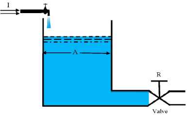
Liquid tank system

The lower and upper bounds of absolute errors.
| α | SNN | DNN | Neural network |
|---|---|---|---|
| 0 | [(0.0435, 0.0994),p(0.72,0.81,0.87)] | [(0.0112, 0.0442),p(0.75,0.82,0.88)] | [(0.0798, 0.1153),p(0.7,0.75,0.85)] |
| 0.2 | [(0.0504, 0.0940),p(0.7,0.8,0.9)] | [(0.0248, 0.0635),p(0.75,0.82,0.9)] | [(0.0878, 0.1375),p(0.7,0.8,0.85)] |
| 0.4 | [(0.0441, 0.0802),p(0.8,0.85,0.92)] | [(0.0131, 0.0422),p(0.8,0.9,1)] | [(0.1105, 0.1592),p(0.75,0.83,0.9)] |
| 0.6 | [(0.0178, 0.0423),p(0.8,0.92,1)] | [(0.0121, 0.0384),p(0.81,0.94,1)] | [(0.0613, 0.0915),p(0.8,0.9,1)] |
| 0.8 | [(0.0608, 0.0709),p(0.71,0.8,0.9)] | [(0.0154, 0.0309),p(0.8,0.87,0.95)] | [(0.0739, 0.0925),p(0.7,0.8,0.85)] |
| 1 | [(0.0611, 0.0611),p(0.75,0.82,0.91)] | [(0.0335, 0.0335),p(0.8,0.87,0.92)] | [(0.1007, 0.1007),p(0.7,0.8,0.9)] |
Solutions of different methods based on Z-numbers
| α | SNN | DNN | Neural network |
|---|---|---|---|
| 0 | [0.0387, 0.0884] | [0.0101, 0.0398] | [0.0701, 0.1012] |
| 0.2 | [0.0451, 0.0841] | [0.0225, 0.0575] | [0.0771, 0.1207] |
| 0.4 | [0.0407, 0.0740] | [0.0125, 0.0401] | [0.1001, 0.1442] |
| 0.6 | [0.0169, 0.0402] | [0.0115, 0.0365] | [0.0582, 0.0868] |
| 0.8 | [0.0544, 0.0635] | [0.0144, 0.0289] | [0.0649, 0.0812] |
| 1 | [0.0554, 0.0554] | [0.0311, 0.0311] | [0.0901, 0.0901] |
Solutions of different methods based on fuzzy numbers
5. Conclusions
In this paper, two types of Bernstein neural networks are used namely static and dynamic models to approximate the solutions of FDEs on the basis of Z-numbers. Initially the FDE is transformed into four ODEs with Hukuhara differentiability. Then neural models are constructed with the structure of ODEs. With modified back propagation method for Z-number variables, the neural networks are trained. Some real examples are employed to show the effectiveness of the proposed approximation methods with the Bernstein neural networks. The future works are the application of these mentioned methodologies for fuzzy partial differential equations on the basis of Z-numbers.
References
Cite this article
TY  - JOUR
AU  - Raheleh Jafari
AU  - Wen Yu
AU  - Xiaoou Li
AU  - Sina Razvarz
PY  - 2017
DA  - 2017/09/19
TI  - Numerical Solution of Fuzzy Differential Equations with Z-numbers Using Bernstein Neural Networks
JO  - International Journal of Computational Intelligence Systems
SP  - 1226
EP  - 1237
VL  - 10
IS  - 1
SN  - 1875-6883
UR  - https://doi.org/10.2991/ijcis.10.1.81
DO  - 10.2991/ijcis.10.1.81
ID  - Jafari2017
ER  -