
Evaluation of Expert Systems Techniques for Classifying Different Stages of Coffee Rust Infection in Hyperspectral Images
- DOI
- 10.2991/ijcis.11.1.8How to use a DOI?
- Keywords
- Expert systems; Hyperspectral images; Coffee rust infection; Spectral profiles
- Abstract
In this work, the use of expert systems and hyperspectral imaging in the determination of coffee rust infection was evaluated. Three classifiers were trained using spectral profiles from different stages of infection, and the classifier based on a support vector machine provided the best performance. When this classifier was compared to visual analysis, statistically significant differences were observed, and the highest sensitivity of the selected classifier was found at early stages of infection.
- Copyright
- © 2018, the Authors. Published by Atlantis Press.
- Open Access
- This is an open access article under the CC BY-NC license (http://creativecommons.org/licences/by-nc/4.0/).
1. Introduction
It is well known that both physiological and infectious plant diseases can have critical impacts on agricultural production and economic losses worldwide.1,2,3 Common sources of infection include insects and microorganisms such as bacteria, fungi, and viruses. Fungi are the most diverse group of plant pathogens; there are more than 20,000 species of fungi that can cause diseases in crops and plants, and these fungi are responsible for 70–80% of plant diseases.4
Crop loss due to plant diseases may cause food insecurity and famines1; consequently, detecting plant diseases and their pathogens is an operation of primary importance to agricultural field management5,6 and an essential research topic in agriculture.3 Given this scenario, there is a need for research to focus on the rapid design of tools for the early detection of symptoms of a particular disease.3,2 These requirements and the recent developments in agricultural technology have led to a demand for a new era of automated, non-destructive methods for detecting plant diseases.1,2,7
The traditional methods for detecting fungal pathogens in plants involve interpreting the visual symptoms of the disease or identifying the pathogens that cause the disease. To understand the visual symptoms of a particular disease, persons skilled in the disease are used.3,4,5,6 To identify the pathogens that cause a particular disease, morphological, microbiological and biochemical techniques may be used.4
However, visual inspection methods are subjective, occasionally inconsistent and generally slow, and given their high cost, such methods are often prohibitive on large farms. Meanwhile, laboratory analyses, such as molecular, immunological or pathogen culturing-based approaches, are often time consuming and destructive.6,8
In this context, it is compelling to develop non-destructive, automated methods that are capable of identifying diseases in a rapid and reliable way and that are capable of detecting early infections;6,9 thus, new techniques such as digital images that can extract information of symptoms in the visible and near-infrared (NIR) bands are receiving attention.6 In these ranges, according to Refs. 10–12, the spectrum of plant leaves changes in both the visible and the near-infrared regions due to physiological stress. Furthermore, metabolic disturbances were found to affect the ability of chlorophyll to absorb visible light, and with the deterioration of the metabolism, the visible reflectance increases. It was also reported that the reflectance of a leaf in the NIR region decreases in advanced disease infestation as actual breakdown of the leaf occurs. Thus, it is not surprising that methods for automatic plant disease diagnosis based on visible range digital images have received special attention.13,14
Using the spectrum variations according to the health conditions of the plant and the assumption that objects with the same spectral characteristics should belong to the same class and be assigned to one characteristic appearance in the final classification map requires a procedure that assigns each pixel to one of other predefined classes.12 Accordingly, several studies have shown the capabilities of red green blue (RGB), multispectral images (MSIs) and hyperspectral images (HSIs) for detecting fungal diseases in crops, as shown in tablenew.
Hyperspectral imaging is the most powerful technique since it can capture both spectral and imaging information for the same object covering hundreds of wavebands, which allow determining the physical, morphological and chemical characteristics and molecular information of materials. HSIs are formed by a high number of intensity images, commonly named channels, in a three-dimensional array called a hypercube,26 which includes some regions that are not detectable by the human eye, such as ultraviolet, near infrared, and infrared. This characteristic is of considerable interest for its application in precision agriculture2 disease evaluation.4 However, this technique requires the use of special methods, such as those based on machine learning techniques such as artificial neural networks (ANNs), decision tree (DT), K-means (KM), K-nearest neighbor (KNN), and support vector machine (SVM), for data analysis. These techniques have been applied in agricultural research and shown potential for automatic classification methods in site-specific weed detection.7
Yellow coffee rust, which is caused by the fungus Hemileia vastatrix B & B, is one of the most economically important diseases affecting coffee27,28,29; it reduces the photosynthetic activity and causes defoliation of the plant.30 This disease causes worldwide economic losses of approximately $1 billion US dollars due to high mitigation costs and the decrease in productivity of up to fifty percent.28,31 Thus, to prepare mitigation actions, it is necessary to evaluate rust damage during the early stages of infection.32 Therefore, in the diagnosis of plant fungal infections, it is essential to perform a correct disease detection process,4 particularly using non-destructive and real-time techniques.1
Consequently, the main objective of this work was to evaluate the use of expert systems techniques and hyperspectral imaging to classify different stages of coffee rust infection in coffee (Coffea Typica) leaves.
2. Materials and Methodology
2.1. System for acquiring hyperspectral images
The system for acquiring hyperspectral images was obtained from RESONON Inc., model PIKA XC (see fig 1).
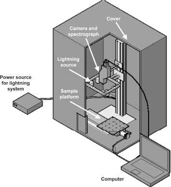
Hyperspectral imaging system.
The elements that compose the system for hyper-spectral image acquisition are as follows:
- •
Camera and spectrograph. Filtering of the wavelengths at which to acquire the intensity images.
- •
Cover. To avoid the influence of exterior lighting.
- •
Computer. To manage the image acquisition software.
- •
Power source. Provides energy for light source.
- •
Light source. Composed of four halogen lights arranged at variable and adjustable height.
- •
Sample platform. For horizontal scrolling during speed-controlled scanning.
This system operates in a reflectance mode with scanning line by line (pushbroom) in the range of 400 – 1,000 nm, obtaining intensity images at intervals of 8 nm (76 images per scene). These images are arranged in a three-dimensional matrix, called a hypercube,26 whose extension is “.bil” (band interleaved by line) and requires a header file whose extension is “.hdr”.
2.2. Samples
The sample was composed of 140 coffee leaves (var. Typica); these leaves were collected from a coffee plantation located in the district of San Nicolas, province of Rodríguez de Mendoza in the Amazons region [-6.40144, -77.50135 U.T.M.]. The sample contains healthy leaves and diseased leaves at different levels of infection with rust. table 1 shows the sample, and in fig 2, the progression of rust infection in coffee leaves is shown as a reference.
| State | Disease/Pest | Technique | Model | Wavelength (nm) | Results (accuracy %) | Source |
|---|---|---|---|---|---|---|
| Eggplant leaves | Botrytis cinerea | HSI | ANN | 400 – 900 | 70.5 | Ref. 15 |
| Rice leaves | Helminthosporium oryzae | HSI | RA | 400 – 2,350 | 96 | Ref. 5 |
| Citrus | Penicillium digitatum | HSI | NLBDA | 400 – 1,800 | 97 | Ref. 16 |
| Maize kernel | Fusarium | HSI | PLS-DA | 1,000–2,498 | 85 | Ref. 17 |
| Rice panicles | Phoma sorghina | HSI | ANN | 350 – 2,500 | > 91 | Ref. 18 |
| Leafs | Sclerotinia | RGB | ANN | – | > 96 | Ref. 3 |
| Cotton | Phymatotrichum omnivorum | HSI - MSI | ISODATA | 400 – 1,000 | > 96 | Ref. 19 |
| Wheat leaves | Fusarium | HSI | SAM | 400 – 1,000 | 87 | Ref. 20 |
| Wheat leaves | Blumeria graminis | HSI | MLR / PLSR | 450 – 950 | > 90 | Ref. 21 |
| Wheat | Fusarium | HSI | PLS-DA | 1,000 – 1,700 | > 91 | Ref. 8 |
| Wheat leaves | Puccinia striiformis | Spectroradiometer | PLSR | 350 – 2,500 | > 89 | Ref. 22 |
| Sugar beet | Cercospora beticola | RGB | SVM | – | > 93 | Ref. 23 |
| Wheat kernels | Fusarium | MSI | MLR | 360 – 950 | – | Ref. 24 |
| Tomato leaves | Alternaria solani - Phytophthora infestans | HSI | ELM | 380 – 1,023 | > 97 | Ref. 25 |
| Strawberry leaves | Collectotrichum gloeosporidides | HSI | SAM / SDA / CM | 460 – 930 | > 80 | Ref. 1 |
RA = Ratio Analysis; NLBDA = Non-linear Bayesian Discriminant Analysis; PLS-DA = Partial Least Squares and Discriminant Analysis; ISODATA = Iterative Self-Organizing Data Analysis; LDA = Linear Discriminant Analysis; MLR = Multiple Linear Regression; PLSR = Partial Least Squares Regression; ELM = Extreme Learning Machine; SAM = Spectral Angle Mapper; SDA = Stepwise Discriminant Analysis; CM = Correlation Measure.
Evaluation of fungal diseases using image analysis coupled to spectroscopic technology.
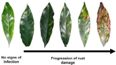
Progression of rust infection in coffee leaves.
2.3. Methodology
The methodology proposed in this research is based on the methods proposed by Refs. 1, 32, and 33. This methodology focuses on the generation, validation, and comparison of classifiers, and it is described in fig 3.
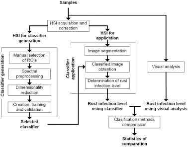
Experimental methodology.
In the following subsections, the stages and steps used are explained in detail.
2.3.1. HSI acquisition and correction
First, the system parameters for HSI acquisition were set as follows: speed of sample platform = 0.5 cm/s, distance to sample surface = 28.3 cm, and diaphragm aperture = 6.4 mm. Then, using the software SpetrononPro 2.62, the hyperspectral images of each leaf were obtained.
Subsequently, the HSIs were spatially corrected according to the methods proposed by Refs. 34, 35, and 36. For this purpose, eq01 was used, and the values of white reference image intensity (W) were acquired from a Teflon pattern (reflectance value of ~99.9%), and the black reference (D) was acquired by blocking the lens (reflectance of ~0.0%).
Here, Pij is the value of the pixel at position (ij) in the raw image I(x,y,λ) at all wavelengths ( λ). P′ij is the pixel value in the corrected image I′(x,y,λ), Dij is the value of the pixel in the black reference image, and Wij is the value of the pixel in the white reference.
2.3.2. Classifier generation
At this stage, three classifiers were generated using spectral information from the different levels of disease progression; the steps followed are detailed below.
Manual selection of regions of interest (ROIs). In each leaf, by using its image in RGB format, ROIs were selected based on the visual appearance. For this purpose, five levels of rust infection and its visual signs were pre-established; see fig4tableand fig4.
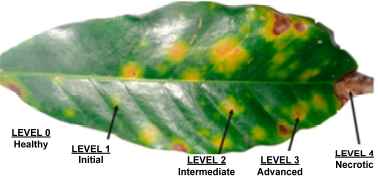
Example of visual signs for rust infection in coffee leaves.
Spectral profiles of each level of damage were obtained using the ROI selection method proposed by Ref. 20, which is summarized in fig 5, and a graphical user interface (GUI) developed and implemented for this purpose in Matlab 2015a. This GUI used the position of each pixel in manually selected ROIs correlating with its levels of rust infection.
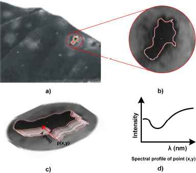
(a) Section containing ROI; (b) Increase of section; (c) Manual drawing of ROI; (d) Obtaining spectral profiles.
This method is compared with the works of Refs. 37, 38, and 39 based on the selection of rectangular ROIs or with the methods used by Refs. 40 or 41 based on a difference in contrast, allowing different stages in tissues to be followed and improving information for the training of classifiers.
However, because this method could generate errors through the border effect or irregular distribution of damage levels in the selected tissue, it is necessary to pre-process the spectral profiles to reduce noise and remove anomalous profiles.
Spectral preprocessing. In most cases, the extracted spectral data contain some noise and variability, and addressing this variability requires the use of spectral enhancement, such as spectral filtering, smoothing, normalization, mean centering, and auto scaling.12
For this research, the spectral profiles were first smoothed using a second-degree Savitzky-Golay filter; see eq.2.
Here, Y is the original profile, Yo is the filtered profile, C is the coefficient for the ith term of the profile, and N is the number of convolution integers.
Subsequently, anomalous spectral profiles were removed using a script that evaluates intensity values at each wavelength and deletes those whose intensity deviates from the median by more than one standard deviation. This script uses the following steps:
- (i)
Select wavelength (λi).
- (ii)
Calculate the median (Î) and standard deviation (σ1) of the intensity value at (λi).
- (iii)
Select a profile (p).
- (iv)
If Ip < Î − σI or Ip > Î + σI, delete profile (p); otherwise, keep profile (p).
- (v)
Return to point (item iii) until finishing the profiles.
- (vi)
Return to point a until the wavelengths are over.
Dimensionality reduction. In many situations, dimensionality reduction can improve model performance and model characteristics by identifying and removing useless, noisy and redundant variables.42 Therefore, in this research, the possibility of dimensionality reduction was evaluated using the Bartlett test and Kaiser-Meyer-Olkin (KMO) test. Subsequently, following the reports of Refs. 43, 44, 45, and 46, the dimensionality of the input data was reduced using principal component analysis (PCA).
PCA reduces the dimensions of the data, transforming the initial dimensions into new uncorrelated dimensions called main components through a linear combination of the initial dimensions, and these are obtained in order of importance according to their capacity to represent the greater variability of the data.43 This step was performed using the pca function of Matlab 2015a.
Creation, training and validation of classifiers. Using the Matlab 2015a classification learner toolbox, three different classifiers were created and trained: support vector machine (SVM), decision tree (DT), and K-nearest neighbor (KNN).
From each classifier, confusion matrices and the principal statistics values were obtained to select the classifier with the best performance.
2.3.3. Classifier application
At this stage, the potential of the expert system previously selected to determine the progress of leaf rust infection was evaluated in comparison to the visual analysis performed by experts.
The first step was the segmentation of the images. In this step, the pixels of the image containing coffee leaf information were selected using the contrast between the sample and background; see eq.7.
Here, g is the binary image, p(x,y) represents the intensity of the image in gray scale, and T is the threshold. In this step, intensity images were selected at 562 nm because greater contrast between sample and background exists at this wavelength; see fig 6.
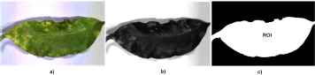
Leaf image: a) RGB, b) 562 nm, and c) segmented.
To obtain classified images, according to the level of damage in the coffee leaves, a pixel by pixel analysis is conducted to determine the affected area over the entire sample. For this purpose, the position of the sample pixel and its spectral profile are obtained, and then eq.8 is used to determine the state of damage.
Here, H is the classified image, C is the classifier, I(x,y) is the spectral profile, and g is the segmented image.
Next, we proceed to determine the percentage of leaf area with rust (PLAR) quantifying the number of pixels per state of damage; see eq.9 .
Here, PLAR is the percentage of leaf area with rust, i are the levels of rust damage, and N is the number of pixels.
2.3.4. Visual analysis
To conduct the visual analysis (VA), judges belonging to The Phytopathology Laboratory of the Research Institute for the Sustainable Development of Ceja de Selva at National University Toribio Rodríguez de Mendoza of Amazons were used; these judges performed the visual analysis of samples using the SAGARPA scale; see table 2.
| State | Number of leaves for classifier | |
|---|---|---|
| Generation | Application | |
| Healthy | 5 | 12 |
| Sick | 15 | 108 |
| Total | 20 | 120 |
Distribution of the coffee leaves that composed the sample.
2.3.5. Classification method comparison
In this stage, the results of the classification of validation samples using the trained classifiers and visual classification were compared; it was determined whether there are statistically significant differences between the classification techniques, and the classification method that presents the greatest performance was identified.
3. Results and Discussion
3.1. Preprocessing phase
In the first steps of the methodology, a total of 22,498 profiles distributed in the pre-established levels were obtained. These profiles were smoothed, the median was extracted, and the upper and lower bounds were determined by adding and subtracting the standard deviation. These profiles are plotted in fig 7a.
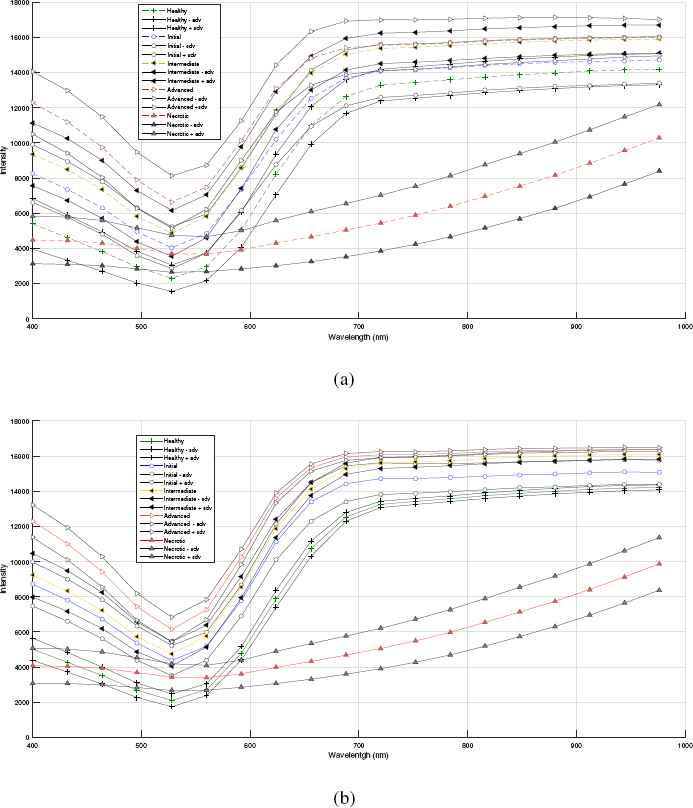
Spectral profiles (a) without removal of outliers and (b) with removal of outliers.
However, this graph shows excessive overlap between levels that, as commented in Ref. 6, may be due to the manual selection of ROIs, which could have a large impact on the features extracted to describe these regions and logically on the detection accuracy.
Consequently, it was necessary to perform correction by removing the outliers, and the results are plotted in fig 7b, which shows that the median profiles with or without outliers are the closest, but in the second graph, there is a marked reduction in overlap between levels.
3.2. Spectral profiles
The previously obtained median profiles, plotted in fig 8, show a constant pattern throughout the development of the infection. In this case, the median profiles, except for the necrotic stage, show intensity values that are progressively higher during the progression of the infection.
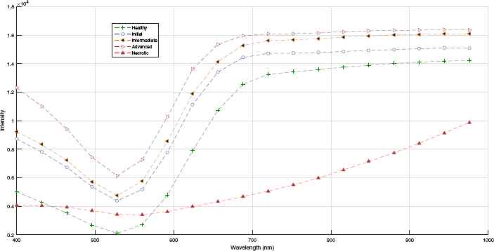
Average spectral profiles of damage caused by rust.
In the initial stages of infection, the profiles show a reduction in intensity from 400 to 530 nm and then an increase in intensity to 670 nm. From this wavelength and up to 1,000 nm, the rate of increase in intensity is slightly lower as the infection progresses. The profile of necrotic tissues, unlike the profiles for the initial, intermediate and advanced stages, starts below the profile for healthy tissues and shows a very low rate of change, similar to that reported by Ref. 19. From the observation of these profiles, it was determined that there is a correspondence between the change in the profiles and the progression of the disease, thereby enabling the analysis of patterns for the later implementation of classifiers.
3.3. Dimensionality reduction
Using the Bartlett test, p-value = 0, it was determined that there is a statistically significant difference between the standard deviations of the wavelengths at 99.0% confidence; likewise, the factor obtained using the Kaiser-Meyer-Olkin test, 0.9813, shows that it is possible and advisable to perform wavelength factorization.
When performing PCA, it was determined that more than 99.1% of the variance could be explained by two components; see fig 9.
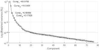
Variance explained by component.
Plotting the score of the two selected components, as shown in fig 10, it is observed that, except for the profiles with necrotic damage, there is a slight confusion in the limits of each level of damage.
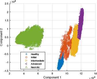
Levels of infection and components.
3.4. Classifier creation, training and validation
The performance of the classification techniques previously mentioned and trained with the two main components determined in the previous step was calculated, and the results are presented in table 3.
| Level | Stage | Visual appearance of tissue |
|---|---|---|
| 0 | Healthy | Characteristic color |
| 1 | Initial | Small round chlorotic spot, diffuse edges |
| 2 | Intermediate | Chlorotic border spot defined |
| 3 | Advanced | Chlorotic spot with initial signs of necrosis, brown coloration |
| 4 | Necrotic | Brown fabrics |
Visual scale for rust infection level in coffee leaves.
The classification techniques used in this paper to differentiate the five stages of rust infection showed precisions between 90 and 94.7%. These results are similar to previously reported results and those shown in table 1 for fungal diseases with signs in leaves. In this work, the obtained results were slightly superior to those obtained by Refs. 1 and 48, who classified three stages of anthracnose infection in strawberry leaves and Fusarium infection in wheat leaves, respectively, but the results were slightly inferior to those reported by Ref. 25 in evaluating tomato leaf infection by Alternaria solani and Helminthosporium oryzae infection over rice leaves.5
When analyzing the techniques used in detail through the confusion matrices shown in table 3, we observe the following:
- •
The technique that obtained the highest accuracy (94.7%) and lowest error (5.3%) was SVM.
- •
The decision tree technique obtained the lowest rate of false positives.
- •
According to the MUAC indicator (an indicator of the performance level of the classifier), the three techniques used showed good performance, with a range between 83 and 96%.
- •
Referring to the classification between classes, shown in fig 11, except for the initial state, the different stages of progression of the infection can be classified using the techniques at an average percentage accuracy of 97.6%.
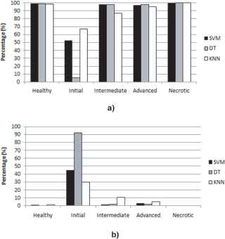
ACC and ERR when classifying states of damage. a) ACC and b) ERR.
Based on the results of the ACC, ERR, FP and MAUC metrics, the classifier to be used in the experimentation phase was selected. Consequently, the SVM technique is the one that achieves better benefits for our case study.
3.5. Classifier application
The coffee leaves were analyzed following the guidelines shown in section 2.3.3. For this purpose, the previously trained classifier (SVM) was used, its PLAR was determined, and its respective classified image was generated. fig 12 presents an example of the use of the SVM technique in our case study.
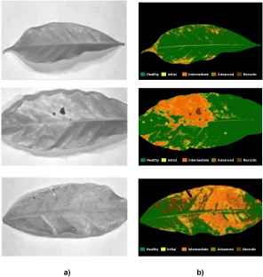
Classification of rust infection states: a) Intensity images and b) classified images.
From the PLAR value and the limits for leaf damage levels established by SAGARPA, as shown in table 2, the classification of the validation samples was performed, obtaining different degrees of infection. fig 13 shows the results for each method used; as shown, there are differences in the results of the applied methods.
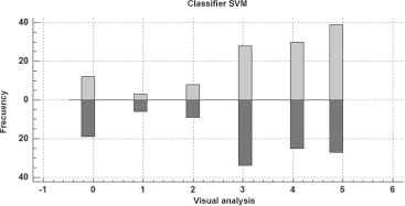
Frequency of classes obtained by the SVM classifier and visual analysis.
3.6. Evaluation of classification methods
Due to differences in the results of the applied methods (SVM and VA), it is necessary to determine whether such differences are significant. For this purpose, a non-parametric statistical analysis was performed using the Kolmogorov-Smirnov test. Consequently, it was determined that there are statistically significant differences. table 4 shows the results of the Kolmogorov-Smirnov test in detail.
| Level | Description | PLAR |
|---|---|---|
| 1 | Slightly visible chlorotic spots | 0.5 – 1 |
| 2 | Visible symptoms of leaf area | 1 – 5 |
| 3 | The stains begin to bond | 6 – 20 |
| 4 | The leaves begin to show obvious necrosis | 21 – 50 |
| 5 | High percentage of necrotic areas | > 50 |
Source: extracted from SAGARPA.47
Scale for evaluating rust advance level.
Subsequently, through the Wilcoxon signed-rank test, the method that generates the highest class values was determined. table 5 presents the results of the Wilcoxon test.
| Support Vector Machine | |||||||
| Healthy | Initial | Intermediate | Advanced | Necrotic | Metrics* | ||
| Healthy | 99.20% | 0.80% | 0.00% | 0.00% | 0.00% | ACC: | 94.70% |
| Initial | 2.90% | 52.40% | 44.70% | 0.00% | 0.00% | ERR: | 5.30% |
| Intermediate | 0.00% | 0.00% | 98.50% | 1.50% | 0.00% | PRC: | 95.30% |
| Advanced | 0.00% | 0.00% | 3.10% | 96.90% | 0.00% | FP: | 0.60% |
| Necrotic | 0.00% | 0.00% | 0.00% | 0.00% | 100.00% | MAUC: | 96.00% |
| Decision Tree | |||||||
| Healthy | Initial | Intermediate | Advanced | Necrotic | Metrics* | ||
| Healthy | 99.10% | 0.00% | 0.00% | 0.00% | 0.00% | ACC: | 90.30% |
| Initial | 2.60% | 5.50% | 91.80% | 0.00% | 0.00% | ERR: | 9.70% |
| Intermediate | 0.00% | 0.00% | 98.10% | 1.90% | 0.00% | PRC: | 90.70% |
| Advanced | 0.00% | 0.00% | 2.10% | 97.90% | 0.00% | FP: | 0.50% |
| Necrotic | 0.00% | 0.00% | 0.00% | 0.00% | 100.00% | MAUC: | 86.00% |
| K-Nearest Neighbor | |||||||
| Healthy | Initial | Intermediate | Advanced | Necrotic | Metrics* | ||
| Healthy | 98.70% | 1.30% | 0.00% | 0.00% | 0.00% | ACC: | 93.00% |
| Initial | 2.80% | 67.10% | 30.10% | 0.00% | 0.00% | ERR: | 7.00% |
| Intermediate | 0.00% | 10.50% | 87.20% | 2.30% | 0.00% | PRC: | 96.30% |
| Advanced | 0.00% | 0.00% | 5.00% | 95.00% | 0.00% | FP: | 3.40% |
| Necrotic | 0.00% | 0.00% | 0.00% | 0.00% | 100.00% | MAUC: | 83.00 |
ACC: Accuracy; ERR: Error; PRC: Precision; FP: False positive; MAUC: Minimum area under curve.
Confusion matrices for classification techniques.
Meanwhile, from the statistics for the VA-SVM ratio, shown in table 6, it is observed that there is a statistically significant difference between the VA and the SVM (p = 0.000 < 0.05–Wilcoxon test). In addition, it was determined that the SVM ratings are significantly higher than those obtained by VA.
| Statistical | Classifier SVM | Visual Analysis | |
|---|---|---|---|
| N | 120 | 120 | |
| Normal parameters(a) | Media | 3.49 | 3.01 |
| Standard deviation | 1.55 | 1.68 | |
| Absolute | 0.21 | 0.22 | |
| More extreme differences(b) | Positive | 0.17 | 0.12 |
| Negative | −0.21 | −0.22 | |
| The Kolmogorov-Smirnov Z | 2.32 | 2.35 | |
| Asymp.sig. (2-tailed) | 0 | 0 | |
The contrast distribution is normal.
Data from both variables are normal (0.00 ⩾p < 0.05).
Kolmogorov-Smirnov test for classification.
Finally, the statistics of both methods were evaluated using samples with a PLAR between 0 and 0.5 and a total of 12 leaves; see table 7.
| Visual - SVM | N | Average rank | Sum of ranks |
|---|---|---|---|
| Negative rank | 52(a) | 27.07 | 1 407.50 |
| Positive rank | 1(b) | 23.5 | 23.5 |
| Draws | 67(c) | ||
| Total | 120 | ||
Visual < SVM.
Visual > SVM.
Visual = SVM.
Wilcoxon signed-rank test.
From these data, it was determined using a Student t-test 0.000 ⩽ p < 0.05 at a 95% confidence level that there is a significant difference between the PLAR obtained with the SVM and the minimum observed with VA. table 8 presents the results.
| Statistical | Visual - SVM |
|---|---|
| Z | −6.687(a) |
| Asymptotic Sig. (bilateral) | 0.000(b) |
Based on positive ranges.
Based on the Wilcoxon signed-rank test.
The contrast statistics for the VA-SVM ratio.
In this way, there is sufficient statistical evidence to confirm that the rigor of evaluation using an expert system based on an SVM classifier is more rigorous than that using VA and the SAGARPA scale. Therefore, it is necessary to develop a new scale for the proposed methodology to increase the effectiveness of rust treatment in coffee plants.
| N | Median | Standard deviation | Standard Error |
|---|---|---|---|
| 12 | 0.1167 | 0.103 | 0.030 |
Statistics of the sample PLAR.
| t | gl | Sig. (bilateral) | Difference of means | Confidence interval for the difference | (95%) |
|---|---|---|---|---|---|
| lower | upper | ||||
| −12.894 | 11 | 0.000 | −0.38333 | −0.4488 | −0.3179 |
T-test for a sample.
4. Conclusions
In this paper, we investigated the potential of using expert systems techniques for classifying different stages of coffee rust infection in hyperspectral images. Five levels of infection were preestablished (healthy, initial, intermediate, advanced and necrotic), which were used to create and train three classifiers (DT, SVM, and KNN). The results of the experiment revealed differences in their mean spectral profiles. The classifier based on the SVM technique obtained the best classification performance (ACC = 94.7%, and FP = 0.6%). The results obtained using the SVM classifier were statistically compared against the results obtained through visual analysis, and a statistically significant difference was observed. The results have confirmed the feasibility of using expert systems techniques and hyperspectral images for evaluating the progression of coffee rust infection.
Acknowledgments
This work has been funded by the Fund for Innovation, Science, and Technology (FINCyT) through the Project Contract 220-IA-2013. The fourth author thanks CONACYT-Mexico for the support to participate in this research work through project 2143-Fortalecimiento de las capacidades de TICs en Nayarit.
References
Cite this article
TY  - JOUR
AU  - Wilson Castro
AU  - Jimy Oblitas
AU  - Jorge Maicelo
AU  - Himer Avila-George
PY  - 2018
DA  - 2018/01/01
TI  - Evaluation of Expert Systems Techniques for Classifying Different Stages of Coffee Rust Infection in Hyperspectral Images
JO  - International Journal of Computational Intelligence Systems
SP  - 86
EP  - 100
VL  - 11
IS  - 1
SN  - 1875-6883
UR  - https://doi.org/10.2991/ijcis.11.1.8
DO  - 10.2991/ijcis.11.1.8
ID  - Castro2018
ER  -