
Missing values estimation and consensus building for incomplete hesitant fuzzy preference relations with multiplicative consistency
- DOI
- 10.2991/ijcis.11.1.9How to use a DOI?
- Keywords
- Hesitant fuzzy preference relation; Incomplete hesitant fuzzy preference relation; Multiplicative consistency; Group decision making; Consensus
- Abstract
This paper proposes a decision support process for incomplete hesitant fuzzy preference relations (HFPRs). First, we present a revised definition of HFPRs, in which the values are not ordered for the hesitant fuzzy element. Second, we propose a method to normalize the HFPRs and estimate the missing elements in incomplete HFPRs based on multiplicative consistency. Based on this, a consensus model with incomplete HFPR is developed. A feedback mechanism is proposed to obtain a best choice with desired consensus level. Multiplicative consistency induced ordered weighted averaging (MC-IOWA) operator is used to aggregate the individual HFPRs into a collective one. A score HFPR is proposed for collective HFPR, and then the hesitant quantifier-guided non-dominance degrees (HQGNDD) of alternatives by using an OWA operator are obtained to rank the alternatives. Finally, a case study for evaluate the qualification of supply chain enterprises is provided to illustrate its application.
- Copyright
- © 2018, the Authors. Published by Atlantis Press.
- Open Access
- This is an open access article under the CC BY-NC license (http://creativecommons.org/licences/by-nc/4.0/).
1. Introduction
As a new extension of fuzzy sets, Torra1 proposed the concept of the hesitant fuzzy set (HFS), which permits the membership degree of a given element to be described as several possible values between 0 and 1 and that is called hesitant fuzzy element (HFE). Due to the advantages of handing imprecision by two or more sources of vagueness appear simultaneously2, HFSs have attracted great attention by researchers and have been widely applied in decision making3,4,5,6. Rodríguez et al.7 extended the HFSs to linguistic environment, and introduced hesitant fuzzy linguistic term set (HFLTS). Rodríguez et al.8 provided an overview of the fuzzy linguistic approached for modelling complex linguistic preferences and gave some proposals for future research. Dong et al.9 proposed a novel computing with words (CW) methodology where the HFLTS can be constructed based on unbalanced linguistic term sets (ULTSs) using a numerical scale. Motivated by the concept of HFS, and using Saaty10’s 1/9-9 scale to denote the preference degrees, Xia and Xu11 introduced hesitant multiplicative set (HMS).
As a basic tool to collect and present preferences, the preference relations have been widely used. For example, multiplicative preference relation10,12, interval fuzzy preference relation13, linguistic preference relation14, intuitionistic fuzzy preference relation15, etc. Xia and Xu11 first proposed the concept of hesitant fuzzy preference relation (HFPR), which provided a precise description of the decision makers’ (DMs’) hesitation in providing their preferences. Till now, numerous types of preference relations have been proposed: complete/incomplete HFPRs16,17,18,19,20, hesitant fuzzy linguistic preference relation21, and hesitant multiplicative preference relation.
Thereafter, multi-attribute decision making problems were studied. Zhu et al.2 explored the ranking methods with HFPRs in the group decision making (GDM) environments. Liao et al.22 investigated the multiplicative consistency of HFPRs and its application in GDM. There are so many researches have been developed for the complete hesitant preference relations. However, in many real decision making problems, due to time pressure, lack of knowledge, and DM’s limited expertise related with the problem domain, the DMs may offer a preference relation with incomplete information23,24,25, i.e., some of the pairwise comparison information is missing. Xu et al.17 called the HFPR with some entries are unknown incomplete HFPR, and developed two goal programming models to derive the priority weights from an incomplete HFPR based on multiplicative and additive consistency respectively. Zhang16 established two goal programming for deriving the priority weights from incomplete HFPR based on α-normalization and β-normalization respectively. Zhang et al.18 proposed an algorithm to estimate the missing values and solve the multi-criteria GDM problem with incomplete HFPRs. As far as we know, there are only above three papers which concentrate on the incomplete HFPR. Therefore, it is important to pay attention to this issue. The first objective of the paper is to estimate the missing values for incomplete HFPRs.
Furthermore, there are some limitations for the existing definition of the HFPRs. First, the values in the HFEs are generally arranged in ascending or descending order, which may distort DMs’ original information. Second, since the numbers of values in different pairwise comparisons are generally not identical, in order to operate correctly, a normalization process, such as β-normalization, is carried out, in which some additional values are added into the original set. However, the added values are randomly, and the normalization processes are artificially, which are commented by Rodríguez et al.26. Therefore, the second objective of the paper is to redefine the concept of HFPRs and propose another normalization method. In the final GDM, it generally requires that all the DMs reach a predefine consensus threshold to ensure the final decision is satisfied. Many consensus models have been constructed to explore the consensus level with different preference relations27,28,29,30,31. Dong et al.32 developed an optimization-based consensus model in the hesitant linguistic GDM, which minimizes the number of adjusted simple terms in the consensus building. However, there is no consensus research for the incomplete HFPRs. This motived us to propose a consensus model to deal with incomplete HFPRs. This is the third objective of the paper.
In this paper, we propose a new principle based on multiplicative consistency to normalize the HFPRs. When the DMs provide the preference relations with missing values, one way is to estimate the unknown values. Thus, we provide a way to estimate the missing values in incomplete HFPRs which is based on multiplicative consistency. Thereafter, we develop a GDM process for incomplete HFPRs, which is related with consistency degree and consensus level. Feedback mechanisms is proposed to give personalized advice to DMs, whose consensus level is below the threshold value. Moreover, a multiplicative consistency induced ordered weighted averaging (MC-IOWA) operator is introduced to aggregate all the DMs’ HFPRs into a collective HFPR. A score HFPR is proposed for collective HFPR, and then the hesitant quantifier-guided non-dominance degrees (HQGNDD) of alternatives by using an OWA operator are obtained to rank the alternatives.
This paper is organized as follows. In Section 2, we briefly review some basic concepts and propose a new definition about HFPRs and normalized HFPRs (NHFPRs). In Section 3, we estimate the missing values in the incomplete HFPRs based on multiplicative consistency, and give an algorism to add elements in the process of normalization. Sections 4 and 5, the concept of consistency index and proximity index are defined. Both of them play a crucial role in the measurement of degree of consensus level. A feedback mechanism is proposed to support experts in changing their opinions to achieve a consensus solution with a high degree of consistency. Section 6, a case study is developed to show how the developed consensus model with incomplete HFPR works for practical problems. Finally, we summarize this paper in Section 7.
2. Preliminaries
In this section, some concepts and results of HFPRs are introduced, which will be used throughout the paper.
2.1. Fuzzy preference relations (FPRs)
For simplicity, we denote N = {1,2,…,n}. Let X = {x1,x2, …, xn} (n > 2) be a set of alternatives, where xi represents the ith alternative. A FPR R = (rij)n×n is described as follows33. The preference information on X is described by a FPR R ⊂ X × X, R = (rij)n×n with membership function μR : X × X → [0,1], where μR(xi,xj) = rij, ∀i, j ∈ N. rij represents the preference degree of alternative xi over xj provided by a DM:
- •
rij = 0.5 indicates the DM’s indifference between xi and xj (xi ∼ xj);
- •
0 ⩽ rij < 0.5 means that xj is preferred to xi (xj ≻ xi), and the smaller rij the stronger the preference of alternative xj over xi;
- •
0.5 < rij ⩽ 1 implies that xi is preferred to xj (xi ≻ xj), and the greater rij the stronger the preference of alternative xi over xj.
Definition 1 34.
Let X = {x1, x2, … xn} be a set of alternatives, then R = (rij)n×n is called a FPR on X × X with the following conditions:
Definition 2 33.
Let R = (rij)n×n be a FPR, then it is called a multiplicative consistent FPR if and only if
Remark 1.
In some case, additive transitivity property is in conflict with the [0,1] scale used for providing the preference values. Moreover, Chiclana et al.35 have verified that multiplicative transitivity property is the most appropriate property to model and measure consistency of reciprocal preference relations. In this paper, multiplicative consistency is used.
2.2. Hesitant fuzzy set
Torra1 initially proposed the concept of HFSs to deal with the situations in which several values are possible for the definition of the membership of an element.
Definition 3 1.
Let X = {x1,x2,…xn} be a fixed set, a HFS on X is in terms of a function that when applied to x returns a subset of [0,1], which can be represented by the following:
Given three HFEs h, h1, h2, Torra1 defined some operations:
- (1)
- (2)
- (3)
- (4)
- (5)
Let #h denote the number of elements in the HFE h. In most cases, the numbers of possible values in different HFEs are generally different. In order to operate correctly when comparing them, one of the method is to make sure that they have the same number of elements36. To solve this issue, Zhu and Xu37 gave two opposite normalization principles: 1) α-normalization, remove some elements from h, which has more number of elements. 2) β-normalization, add some elements to h, which has fewer elements.
For the β-normalization, Zhu et al.2 introduced the following method to add some elements to a HFE.
Definition 4 2.
Assume a HFE, h = {hσ(s)|s = 1,2,…,#h}, let h+ and h− be the maximum and minimum elements in h respectively. And ξ(0 ⩽ ξ ⩽ 1) be an optimized parameter, then we call h = ξh+ + (1 − ξ)h− an added element.
ξ is used to reflect the DMs’ risk preference. Especially, Xu and Xia36 introduced that ξ = 0 indicates the pessimists expect unfavorable outcomes; ξ = 1 indicates the optimized desirable outcomes.
Definition 5 3.
For a HFE h,
2.3. Hesitant fuzzy preference relations (HFPRs)
Based on the concepts of HFS and FPRs, Zhu and Xu38 proposed the concept of HFPR as follows:
Definition 6 38.
Let X = {x1,x2,…xn} be a fixed set, a HFPR H on X is denoted by a matrix H = (hij)n×n ⊂ X × X, where
Definition 7 2.
Let H = (hij)n×n be a HFPR and an optimized parameter ξ(0 ⩽ ξ ⩽ 1), where ξ is used to add some elements to hij (i < j), and 1−ξ is used to add some elements to hji (i < j), then we obtain a HFPR
Where
Definition 8 2.
Assume a HFPR H = (hij)n×n and its NHFPR
Theorem 1. 16
Given a HFPR H = (hij)n×n, and its NHFPR
- (i)
H is multiplicative consistent;
- (ii)
- (iii)
Theorem 2. 2
Assume a HFPR H = (hij)n×n and its NHFPR
Then, mH = (mhij)n×n is called multiplicative consistent HFPR with ξ.
Remark 2.
Generally, for the HFPR H = (hij)n×n, each preference degree in hij is a possible value, H can be directly separated into all possible FPRs. Thus, the judgement of a HFPR’s consistency is based on the consistency of the corresponding FPRs. In currently researches, it consists of three stages: (1) Normalizing a HFPR H; (2) Dividing a HFPR into several corresponding FPRs in accordance with the number of elements in HFE; (3) Checking the consistency of these corresponding FPRs by Eq. (2). If all of them are consistent, the HFPR is consistent; otherwise, it is inconsistent.
However, there are some problems for the current definitions of HFPRs, as the values in each HFE should be rearranged in ascending or descending order according to Definition 6. This operation may lead to inconsistent. In the following, we will give two examples to show the problems of the Definition 6.
Example 1 16.
Let H be a HFPR, which is shown as follows:
In order to get a multiplicative consistent HFPR mH of H, Zhang16 first normalized it by Definition 7 (where ξ=1), and we have:
By Eq.(9), Zhang16 obtained the multiplicative consistent HFPR mH = (mhij)n×n of H is:
In mH,mh23 = {0.3132,0.3184,0.2949}, its elements do not arrange in ascending order, because 0.2949 is smaller than 0.3132 or 0.3184, which do not meet the requirement
According to Eq.(8), we have
Example 2.
Consider a decision making process of three alternatives X = {x1,x2,x3}, two DMs E = {e1,e2} are invited to give their preference degrees over paired comparisons of alternatives. The result furnishes in Table 1.
| Pair of the three alternatives | Pair-wise judgments | ||
|---|---|---|---|
| Expert 1 | Expert 2 | ||
| x1 versus | x2 | 0.6 | 0.8 |
| x3 | 0.5 | 0.5 | |
| x2 versus | x1 | 0.4 | 0.2 |
| x3 | 0.4 | 0.2 | |
| x3 versus | x1 | 0.5 | 0.5 |
| x2 | 0.6 | 0.8 | |
Experts’ pair-wise judgments.
From Table 1, we know that the first expert e1 gives his preference degrees 0.6 of x1 over x2, 0.5 of x1 over x3, and so on. The second expert e2 gives his preference degrees 0.8 of x1 over x2, 0.5 of x1 over x3, and so on. According to the definition of HFE, the preference degrees of x1 over x2 given these two experts is {0.6,0.8}, and all these values consists of a HFPR Hc as follows:
In order to determine the multiplicative consistency of Hc, according to Definition 8, we only need to verify whether the following two FPRs are multiplicative consistent or not:
Obviously,
However, from the given information of experts e1 and e2 in Table 1, we have their FPRs R1 and R2, respectively:
According to Eq.(2), we can test that both R1 and R2 are multiplicative consistent. For R1, rijrjkrki = rikrkjrji holds for any i, j,k = 1,2,3, i ≠ j ≠ k. For instance, r12r23r31 = 0.6 × 0.4 × 0.5 = 0.12 = r13r32r21 = 0.5 × 0.6 × 0.4 = 0.12. Thus, R1 is multiplicative consistent. Similarly, R2 is also multiplicative consistent. But if we combine R1 and R2 into a HFPR Hc, Hc would be inconsistent according to Definition 8.
Remark 3.
From Examples 1 and 2, we can know that the reorder of HFEs have an impact on the consistency judgment of a HFPR. For Example 1, if we use Theorem 1 to get a new consistency HFPR, and reorder the elements according to Definition 6, then the new HFPR may be not multiplicative consistent again according to Theorem 1. If we do not reorder the elements, the new HFPR will not satisfy Definition 6. Therefore, they are contradictory in some cases. For Example 2, we know that the original judgments for e1 and e2 are multiplicative consistent respectively. But if we use Definition 6 to combine the two DMs’ judgments into one HFPR directly, the HFPR is not multiplicative consistent. The main reason is that the reordering of the elements in HFEs, which will distort the DMs’ original information. Therefore, the existing definition for HFPR is problematic. In order to overcome these drawbacks, we will propose revised definitions of the HFPR and NHFPR as follows:
Definition 9.
Let X = {x1,x2,…xn} be a fixed set, a HFPR H on X is denoted by a matrix H = (hi j)n×n ⊂ X × X, where
Where
Definition 10.
Let H = (hij)n×n be a HFPR and an optimized parameter ξ (0 ⩽ ξ ⩽ 1), where ξ is used to add some elements to hij (i < j), and 1−ξ is used to add some elements to hji (i < j), then we obtain a HFPR
Where
Definition 11.
Let H = (hij)n×n be a HFPR and its NHFPR
Theorem 3.
Given a HFPR H = (hij)n×n, and its NHFPR
- (i)
H is multiplicative consistent;
- (ii)
- (iii)
Theorem 4.
Assume a HFPR H = (hij)n×n and its
Remark 4.
The difference between the new definitions of HFPR, multiplicative consistent HFPR, NHFPR and the current definitions are that the new definitions do not arrange the elements in ascending (or descending) order. If we use Theorem 3 to get a multiplicative consistent HFPR, we would not need to reorder the elements, and it still conforms to Definition 9. Moreover, the new definitions can retain the DMs’ original information as much as possible.
3. Incomplete hesitant fuzzy preference relations and missing elements estimation
In real decision making problems, the experts often have their unique characteristics with regard to knowledge, skills and experience. Sometimes the experts might not possess a precise or sufficient level of knowledge of the problem. In this case, a DM would not be able to provide her/his judgments over some pairs of alternatives, so the DM usually provides an incomplete HFPR, i.e., some HFEs of HFPR are missing or unknown. Consequently, we introduce the concept of incomplete HFPR.
3.1. Incomplete hesitant fuzzy preference relations
Definition 12 17.
Let H = (hij)n×n be a HFPR, where
Where
Definition 13.
Let H = (hij)n×n be an incomplete HFPR and an optimized parameter ξ (0 ⩽ ξ ⩽ 1), where ξ is used to add some elements to hij ∈ EV (i < j), and 1 − ξ is used to add some elements to hji ∈ EV (i < j), then we obtain an incomplete
Then, we call
Definition 14.
Let H = (hij)n×n be an incomplete HFPR, if the missing HFEs of H can be estimated by the known HFEs, then H is called an acceptable incomplete HFPR, otherwise, H is not an acceptable incomplete HFPR.
Theorem 5.
Let H = (hij)n×n be an incomplete HFPR, the necessary condition of acceptable incomplete HFPR H is that there is at least one known HFE in each row or column of H except for the diagonal HFE.
3.2. A procedure to estimate the missing elements for incomplete HFPRs
Assume H is an incomplete HFPR, then the missing HFE
The following notation is introduced:
MV is the set of pairs of different alternatives for which the DM cannot provide the judgment with some values, i.e. HFEs are missing.
Remark 5.
For Eq.(20) and Eq.(14), they are both the forms of multiplicative consistency. The difference of them is the range of parameter k. For Eq.(14), it ranges from 1 to n , it is suit to all the HFEs include the unknown elements. However, when some of the elements are missing as in this paper, Eq.(14) does not work. Therefore, we use Eq.(20) to estimate the missing values. In order to obtain a complete HFPR, we develop an algorithm as follows:
| Input: The incomplete HFPR H = (hij)n×n, and an optimized parameter ξ ∈ [0,1]. |
| Output: The complete HFPR. |
| Step 1: Assume that there is an incomplete HFPR, H = (hij)n×n, by Definition 14, we determine whether it is acceptable, if it is acceptable, go to the next step; otherwise, return it to DM to construct a new acceptable HFPR. |
| Step 2: Using Eq.(11) to obtain an incomplete NHFPR with parameter ξ. |
| Step 3: Utilizing Eqs. (18), (19) and (20) to estimate the missing values, and finally we obtain a complete HFPR. |
| Step 4: End. |
Example 3.
Let H = (hij)4×4 be an incomplete HFP shown as follows:
We apply Algorithm 1 to estimate the missing elements:
Step 1: Obviously, H is an acceptable incomplete HFPR.
Step 2: Using β-normalization with ξ = 1, then the iomplete NHFPR is obtained as follows:
Step 3: Estimating the missing elements x using Eqs.(18), (19) and (20), the calculation process of h24 is as follows:
Therefore,
h24 = {0.3,0.2222}.
Similarly, the other missing elements can be obtained:
h34 = {0.6316,0.6316}.
Step 4: The complete HFPR of H is:
Remark 6.
Since the numbers of elements in HFE are often different, two methods α-normalization and β-normalization are introduced in Ref. 37 to make all the HFE have the same number of values. However, there are some problems in normalization process. On the one hand, the principle aims to have same number elements in two HFEs, for β-normalization, the added values are based on the maximum and minimum values of a HFE, and the added values are not the DM’s original preferences. β-normalization is an artificial process. On the other hand, for optimized parameter , it ranges from 0 to 1. There is no rule how to choose the value for it. For example, assume a HFE h12 = {0.5,0.6} and
Example 4 27.
Let H = (hij)4×4 be a HFPR shown as follows:
In order to obtain a NHFPR of H, we also use x denote the added elements. First, H is transformed into the following two FPRs:
Obviously, H(2) is an incomplete and acceptable FPR. These added elements x can be estimated by using intermediate alternative x3, the computation is given below:
After the estimation process is applied, corresponding NHFPR of H is obtained as follows:
Example 5.
Let H = (hij)4×4 be a HFPR, which is shown as follows:
First, H is transformed into the following two FPRs:
For this HFPR, it is different from Example 4. It is a complete and acceptable HFPR, but the corresponding FPR H(2) is unacceptable. The added elements x cannot be calculated immediately. In order to estimate it, we first use β-normalization with ξ = 1 to get an acceptable FPR H(2). Let
Then the other added elements x can be estimated through the known elements.
We can know that MV = {(2,3,2),(3,2,2),(3,4,2), (4,3,2)}, using Eqs.(18), (19) and (20), we elaborate the computation process of the estimated value for
Then
In a similar way, we can calculate the rest of x through the intermediate alternative x1, after the computation is applied, the NHFPR is following:
Remark 7.
In this example, H(2) is an unacceptable incomplete fuzzy preference relation. Xu et al.39 have proposed some methods to deal with unacceptable situations. In this paper, we choose
For Examples 4 and 5, in the process of normalization, we also use x to denote the added element, x is estimated based on multiplicative consistency with the known elements. The calculation process is the same as incomplete HFPR. In the following, we summarize the above process in the following Algorithm 2.
| Input: The original complete HFPR, H = (hij)n×n, an optimized parameter ξ ∈ [0,1] and x denotes the added elements. |
| Output: The NHFPR. |
| Step 1: Assume that there is a complete HFPR |
| Step 2: Let |
| Step 3: Normalizing HFPR through Definition 4, then obtain the acceptable corresponding FPRs. Using x denotes the added elements. |
| Step 4: Estimate the unknown elements x by Eqs.(18), (19) and (20), then a NHFPR is obtained. |
| Step 5: End. |
4. Consistency of hesitant fuzzy preference relations
In this section, we first define the distance between two HFPRs, and then, we propose a consistency index of HFPRs, which is used to measure the consistency degree of the HFPRs.
4.1. Distance measure for HFPRs
Definition 15.
Let
Definition 16.
Let H1 = (hij,1)n×n and H2 = (hij,2)n×n be two HFPRs, their NHFPRs are
4.2. Consistency indexes
In the following, we will propose a process to measure the degree of consistency between an individual HFPR, H = (hij)n×n and its corresponding multiplicative consistent HFPR, mH = (mhij)n×n at the three different levels: pair of alternatives, alternatives and relation.
Level 1: Consistency index of pair of alternatives:
CIij = 1 − d(hij,mhij).
Level 2: Consistency index of alternatives:
Level 3: Consistency index of a HFPR:
5. A consensus model for GDM with incomplete HFPRs
In the process of a GDM problem, there is a set of experts (DMs), each expert provides his/her preference relation, and it is expected to reach a high consensus degree among experts before the final resolution. To solve the GDM with incomplete HFPRs, we can first use multiplicative consistency based procedure to estimate the missing values and normalize these HFPRs. When we get the complete normalized HFPRs, we measure their consistency degrees at three levels. Furthermore, a multiplicative consistency induced ordered weighted averaging (MCIOWA) operator is developed to aggregate the individual HFPRs to a collective one. The weighting vector of MC-IOWA operator is derived by a linguistic quantifier, in which the DM’s consistency degree is considered, the higher consistency degree, the more the weight, and therefore the more contribution to the collective HFPR. Once the group HFPR is obtained, a proximate degree (PD) is computed to measure the agreement degree of each individual to the collective HFPR. The consensus degree which integrates the CI and PD is designed to decide whether the feedback mechanism should be activated to give recommendations to the experts. If the consensus degree is achieved to a predefined level, the selection process is implemented to get the final result.
The consensus model with incomplete HFPRs is illustrated in the following stages: (1) Estimating missing elements and normalization of HFPRs; (2) Calculating consistency indexes; (3) Calculating proximity degrees; (4) Computing consensus levels; (5) Feedback mechanism; (6) Selection process. The first two steps have already been presented in Sections 3 and 4, respectively. The rest stages will be addressed in the following section.
5.1. Computing proximity indexes
In order to measure how close the individual preferences are from the collective preferences, the proximity measure is devised. The collective preferences are obtained by fusing all the DMs’ preferences using the MC-IOWA operator16,40,41, which is an extension of the induced ordered weighted averaging (IOWA) operator42.
Definition 17 42.
An IOWA operator is defined as:
Where w = (w1, w2, …, wm)T is a weighting vector, such that wt ∈ [0,1],
Definition 18.
Let E = {e1, e2,…,em} be a set of DMs, and {H1,H2,…,Hm} be the HFPRs provided by the DMs on a set of alternatives X = {x1,x2,…,xn}. A MC-IOWA operator of dimension m,
Then, the collective HFPR Hc = (hij,c)n×n is computed as follows:
The weights of the MC-IOWA operator are obtained by the following expression:
Where
The linguistic quantifier is a Basic Unit-interval Monotone (BUM) function f: [0,1] → [0,1], such that f(0) = 0, f (1) = 1 and if x > y, then f(x) ⩾ f(y).
Then, the proximity measure can be obtained in the following three levels:
Level 1: Proximity index on pairs of alternatives (xi, xj), which is the similarity degree between one value of individual’s preference and the collective one:
Level 2: Proximity index on alternatives xi, which is average degree of PPij,t on alternative xi:
Level 3: Proximity index on the relation Ht, which is average degree of PAi,t of expert et:
5.2. Computing consensus level
In the consensus reaching process of GDM problems, the consistency/consensus level should be considered to determine when the feedback mechanism should be designed to provide personal recommendations to each expert. Generally, the consistency index and proximity degree should be considered at the same time. In order to do that, a consensus level is defined as follows:
5.3. Feedback mechanism
Consensus reaching process is a dynamic and negotiation process. If there exists any DM’s consensus level smaller the predefined level, the moderator will generate the personalized advices for the DM how to update his/her preferences, which is called feedback mechanism. It has two steps: (1) Identification of the HFEs; (2) Recommendation generation.
1) The preference values identification
In order to improve the consensus level, one way is to modify the DM’s preference values which contribute less to CL. Based on the above three different levels of proximity measures, we determine these levels respectively.
Step 1: Identify the experts EXPCH whose consensus level is lower than the threshold:
Step 2: Identify the alternatives’ ALT whose consensus levels are lower than the threshold for the identified expert EXPCH:
Step 3: Finally, identify the hesitant preference values APS for the identified alternatives:
2) Recommendation generation
When the preference values have been identified, the feedback stage should generate properly recommendations to help the experts to revise their preferences. In the following, an interactive mechanism is offered to the experts how they can update their preferences. For all the identified hesitant fuzzy preference value (t, i, j) ∈ APS of expert t, expert et is suggested to change his/her values to be close to the corresponding group preference value hij:
- •
If
- •
If
- •
If
5.4. Selection process
When the consensus threshold is achieved, a selection process is applied to obtain the final solution. Chiclana et al.43 presented a quantifier guided non-dominance degree (QGNDD) method to derive a final ranking of the alternatives from a given FPR. This methodology is based on the use of the ordered weighted average (OWA) operators44, which is guided by a linguistic quantifier representing the concept of majority to implement in the decision making resolution. The linguistic quantifier is represented mathematically by a basic unit-monotonic (BUM) function f: [0,1] → [0,1], such that f(0) = 0, f(1) = 1 and if x > y, then f(x) ⩾ f(y), which is used to compute the OWA operator weights as follows:
The hesitant quantifier guided non-dominance degree (HQGNDD) associated to the alternative xi, HQGNDDi is defined as follows:
Where hij,p = max{h′ji,c − h′ij,c,0} representing the degree up to which xi is strictly dominated by xj,
The alternatives can be ranked from best to worst according to the ranking of HQGNDDi.
A decision support process for the GDM with incomplete HFPRs is illustrated in Fig. 1. It comprises three stages: (1) Missing values estimation and normalization of HFPRs; (2) Consensus reaching process; (3) Selection process.
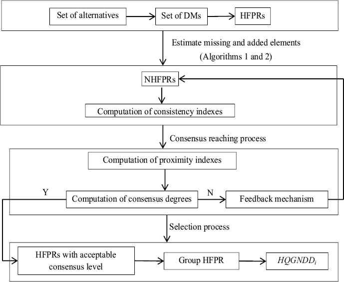
A decision support process for the GDM with incomplete HFPRs
6. A case of study
In this section, the decision support process is applied for qualification of supply chain so as to understand the credit risk of enterprises.
Example 6.
Due to the development of socialized production, the competition between individual enterprises gradually transforms into the competition between supply chains. Upstream and downstream enterprises are extremely important to the core enterprises. Thus, the credit and financing businesses of non-core enterprises have become the first considering factor to the core enterprise. In the existing research results45, we can see that the traditional credit risk evaluation of single enterprise mainly focuses on the qualification of the enterprise. It is influenced by many factors, such as quality of enterprise, credit status, operating capacity, profitability and solvency.
We assume four enterprises xi (i = 1,2,3,4) as alternatives. Three experts E = {e1,e2,e3} are invited to evaluate them. The consensus threshold value η = 0.85. They provide their hesitant preferences over paired comparisons of these four enterprises and give four HFPRs as follows.
In order to help the core enterprise to choose the most suitable enterprise as its upstream enterprise, the following steps are involved:
Step1: Missing values estimation and normalization. y Eqs.(18), (19) and (20), we have:
Step 2: Computing the consistency indexes.
By Eq.(15), we can get the multiplicative consistent HFPR mH for its corresponding HFPR, and then compute the consistency levels: pair of alternatives CIij,t, alternatives CIi,t, and relation CIt.
Level 1: The consistency degrees for each pair of alternatives are:
Level 2: The alternatives consistency levels are:
CIi,1 = (1.0000,1.0000,1.0000,1.0000).
CIi,2 = (0.9328,0.9342,0.9483,0.9523).
CIi,3 = (0.9500,0.9572,0.9817,0.9567).
Level 3: The consistency indexes of individual’s HFPR are:
CI1 = 1.0000, CI2 = 0.9432, CI3 = 0.9614.
In order to get the collective HFPR, we use the BUM function
Step 3: Computing proximate indexes.
Level 1: Proximity indexes PPij,t on pairs of alternatives fo expert et (t = 1,2,3) are:
Level 2: Proximity indexes PPi,t on alternatives for expert et (t = 1,2,3) are:
PPi,1 = (0.9558,0.9542,0.9325,0.9113).
PPi,2 = (0.8223,0.8030,0.7574,0.6333).
PPi,3 = (0.9379,0.9208,0.9352,0.9360).
Level 3: Proximity indexes PPt on the relation for expert et (t = 1,2,3) are:
PP1=0.9385, PP2 = 0.7540, PP3 = 0.9325.
Step 4: Computing consensus levels. Assume δ = 0.5.
Level 1: The consensus levels CLij,t of pair of alternatives for expert et (t = 1,2,3) are:
Level 2: The consensus levels CLi,t of alternatives for expert et (t = 1,2,3) are:
CLi,1 = (0.9779,0.9771,0.9663,0.9557).
CLi,2 = (0.8803,0.8686,0.8529,0.7928).
CLi,3 = (0.9440,0.9390,0.9584,0.9463).
Level 3: The individual consensus levels CLt for expert et (t = 1,2,3) are:
CL1 = 0.9692, CL2 = 0.8486, CL3 = 0.9469.
As the consensus threshold η = 0.85, the feedback mechanism will be activated to assist expert e2 to change his/her preference values due to CL2 = 0.8486 < η.
Step 5: Feedback mechanism.
- (1)
Identify the experts EXPCH: EXPCH = {2}.
- (2)
Identify the alternatives:
ALT = {(2,4)}.
- (3)
The following APS set is obtained:
APS = {(2,4,1),(2,4,2),(2,4,3)}.
Based on the above identified APS, the recommendations for expert e2 are:
You should increase your preference value {0.1,0.3,0.7} for the pair of alternatives (1,4) to a value close to {0.2640,0.5103,0.7780}.
You should decrease your preference value {0.9,0.7,0.3} for the pair of alternatives (1,4) to a value close to {0.7360,0.4896,0.2220}.
You should increase your preference value {0.2,0.3,0.1000} for the pair of alternatives (3,4) to a value close to {0.3935,0.4935,0.3870}.
You should decrease your preference value {0.8,0.7,0.9000} for the pair of alternatives (4,3) to a value close to {0.6065,0.5065,0.6130}.
Your missing preference value for the pair of alternatives (2,4) should be close to {0.4493,0.6311,0.6649}.
Your missing preference value for the pair of alternatives (4,2) should be close to {0.5507,0.3689,0.3351}.
When the expert e2 carried out the changes in his/her HFPR, another round of consensus reaching process will take place.
Assume the expert e2 accepted the recommendations, and his updated values equal to the suggeste values, then the new collective HFPR is:
With the new HFPRs, we compute the consensus levels and have: CL1 = 0.9783, CL2 = 0.8669, CL3 = 0.9504, which are all larger than the predefined threshold η = 0.85, and thus the selection process is applied.
Step 6: Selection process. As H′c is obtained, we apply the proposed HQGNDDi to aggregate the information. By Eq.(27), we have
Using the BUM function
HQGNDD1 = 0.9763, HQGNDD2 = 1.0000,
HQGNDD3 = 0.9196, HQGNDD4 = 0.5774.
According to the degrees HQGNDDi, the ranking of alternatives are:
x2 ≻ x1 ≻ x3 ≻ x4.
Therefore, x2 is the best choice, that is, the credit and financing businesses of x2 is better than other three enterprises. The core enterprise should choose enterprise x2 as its final decision.
In this paper, we first point out the drawbacks of the definition of HFPR for the existing work. Then, we redefine the concept of HFPR, which is slightly different from Zhang16’s definition. The main difference between them is that the HFEs does not need to arrange the elements in ascending (or descending) order in our definition. Furthermore, the new definition can reflect the experts’ original information as much as possible. The existing definition2,5,16,17 needs to arrange the elements in ascending order, which may distort the original preferences. In Example 1, Zhang16 obtained the multiplicative consistent HFPR, in which the element mh23 = {0.3132,0.3184,0.2949}. It is obvious that the values in mh23 are not arranged in ascending order, which is inconsistent with his definition. But if the value of mh23 is arranged in ascending order, mH is not a multiplicative consistent HFPR according his definition. Thus, there exist some issues in current definition, the new definition can avoid this problem.
Second, in the existing literatures (see Ref. 16, 27, 45), β-normalization with ξ = 1 is usually used to obtain NHFPRs, the optimized parameter ξ should be defined in advance, but there is no rule about how to decide the value for it. It is related to the DMs’ risk preference, an optimistic DM and a pessimistic DM may lead to different choice. At the same time, the added elements only relate to the maximum and minimum elements of a HFE, it cannot reflect the DMs’ preference accurately. Therefore, we propose a new normalization method to normalize HFPRs. We look the added value as the missing elements, and use the missing value estimation procedure to estimate these values, and the added values always put after the existing values.
7. Conclusion
In this paper, a GDM with incomplete HFPR is investigated. In order to do this, a new definition of HFPR has been presented. In the normalization process, a new principle to add elements into HFE is put forward. It can accurately reflect the DMs’ original preference and take each element into account, which is important to preserve the DMs’ original as much as possible.
A decision support process is proposed. In order to choosing the best alternative(s), the consensus level is defined, which is related to consistency index and proximity index. A feedback mechanism is activated to support DMs in changing their opinions on condition that the DMs’ consensus level is not reached the threshold value. Once the consensus level is reached, MC-IOWA operator is used to aggregate the individual HFPRs into a collective one. A score HFPR is proposed for collective HFPR, and then the HQGNDD of alternatives are obtained to rank the alternatives. Finally, a case study for evaluate the qualification of supply chain enterprises is provided to illustrate its application.
In this paper, we only use the multiplicative consistency property to estimate the missing values. However, we do not measure its consistency degree. Based on the average-based additive consistency measurement for interval-valued reciprocal preference relations by Dong et al.46, studying the average-based multiplicative consistency for hesitant fuzzy preference relation may be a challenge future work.
Acknowledgments
This work was partly supported by the Key Project of National Natural Science Foundation of China (No. 71633002), the National Natural Science Foundation of China(NSFC) (No.71471056), the Fundamental Research Funds for the Central Universities (No. 2015B23014), sponsored by Qing Lan Project of Jiangsu Province.
References
Cite this article
TY  - JOUR
AU  - Yejun Xu
AU  - Caiyun Li
AU  - Xiaowei Wen
PY  - 2018
DA  - 2018/01/01
TI  - Missing values estimation and consensus building for incomplete hesitant fuzzy preference relations with multiplicative consistency
JO  - International Journal of Computational Intelligence Systems
SP  - 101
EP  - 119
VL  - 11
IS  - 1
SN  - 1875-6883
UR  - https://doi.org/10.2991/ijcis.11.1.9
DO  - 10.2991/ijcis.11.1.9
ID  - Xu2018
ER  -