
A Novel MAGDM Approach With Proportional Hesitant Fuzzy Sets
- DOI
- 10.2991/ijcis.11.1.20How to use a DOI?
- Keywords
- Fuzzy sets; hesitant fuzzy sets; proportional hesitant fuzzy sets; multi-attribute group decision making
- Abstract
In this paper, we propose an extension of hesitant fuzzy sets, i.e., proportional hesitant fuzzy sets (PHFSs), with the purpose of accommodating proportional hesitant fuzzy environments. The components of PHFSs, which are referred to as proportional hesitant fuzzy elements (PHFEs), contain two aspects of information provided by a decision-making team: the possible membership degrees in the hesitant fuzzy elements and their associated proportions. Based on the PHFSs, we provide a novel approach to addressing fuzzy multi-attribute group decision making (MAGDM) problems. Different from the traditional approach, this paper first converts fuzzy MAGDM (expressed by classical fuzzy numbers) into proportional hesitant fuzzy multi-attribute decision making (represented by PHFEs), and then solves the latter through the proposal of a proportional hesitant fuzzy TOPSIS approach. In this process, preferences of the decision-making team are calculated as the proportions of the associated membership degrees. Finally, a numerical example and a comparison are provided to illustrate the reliability and effectiveness of the proposed approach.
- Copyright
- © 2018, the Authors. Published by Atlantis Press.
- Open Access
- This is an open access article under the CC BY-NC license (http://creativecommons.org/licences/by-nc/4.0/).
1. Introduction
The hesitant fuzzy problems are common in daily life, which have been initially interpreted by Torra1 as: “When defining the membership of an element, the difficulty of establishing the membership degree is not because we have a margin of error (as in A-IFS2), or some possibility distribution (as in type 2 fuzzy sets3) on the possible values, but because we have a set of possible values”. To cope with these uncertainties produced by human being’s hesitations, Torra and Narukawa1,5 expanded Zadeh’s fuzzy sets (FSs)6 to another form of fuzzy multi-sets7,8: hesitant fuzzy sets (HFSs). It is worth noting that the HFSs can be applied to describe and handle the following two decision-making cases:
Case 1. Decision is made by one hesitant decision maker, who thinks the membership degree of an object belonging to a concept may have a set of possible values. For example, people’s taste for dessert may change with mood. Good mood may taste more, whereas bad mood may taste less. Therefore, these different tastes constitute a HFS.
Case 2. Decision is made by a team, which contains no less than two decision makers. In this case, the team is automatically divided into more than one group according to the evaluation values of all decision makers: Different groups have distinct opinions on the membership degree, and each group cannot convince each other. For instance, different people may have diverse tastes for dessert, which similarly compose a HFS.
In the aforementioned two cases, the membership degree of an element to a set consists of several possible values in the real unit interval [0,1]. Case 1 derives from the dimension of “time”, whereas “space” dimension is the main factor to promote the second case. Since the introduction of HFSs by Torra and Narukawa1,5, the state-of-the-art regarding HFSs mainly focuses on the following three aspects: aggregation operators, information measures and extensions.
The existing literature on aggregation operators is extensive. Following the intuitionistic fuzzy sets2, Xia and Xu9 defined the hesitant fuzzy weighted averaging operator, hesitant fuzzy weighted geometric operator, and many others. Similarly, a large number of other hesitant fuzzy aggregation operators were defined based on some basic aggregation operators, such as the hesitant fuzzy quasi-arithmetic aggregation operator11, hesitant fuzzy power geometric operators10, induced hesitant fuzzy aggregation operators11 and hesitant fuzzy geometric Bonferroni means12. Especially, in order to alleviate the computational complexity, several improved aggregation principles were also proposed regarding HFSs13,14,15.
The studies of hesitant fuzzy information measures are highly diversified, for instance, the distance and similarity measures on HFSs16,17, correlation coefficients over HFSs18,19 and entropy and cross entropy measures of HFSs20,21. Particularly, Farhadinia21 explored the relationship among them and pointed that the distance, similarity and entropy measures are interchangeable under certain conditions. Furthermore, many extensions on HFSs (for example, the hesitant fuzzy linguistic terms sets22,23, interval-valued hesitant fuzzy sets21,24, higher order hesitant fuzzy sets17 and dual hesitant fuzzy sets25) have also been proposed with the purpose of modeling the hesitant fuzzy problem from various perspectives. Due to the fact that “the hesitant fuzzy set provides a more accurate representation of peoples hesitancy in stating their preferences over objects than the fuzzy set or its classical extensions”10, it has been widely and successfully applied to different practical areas, such as clustering analysis18,26, decision making19,22, and many others.
However, HFSs, including their extensions as mentioned above, are not applicable to addressing the case that a team could not reach agreement on a fuzzy decision (see Case 2), and the proportions of the associated membership degrees are measurable. For example, supposing a decision-making team consisted of ten members is invited to evaluate the membership degree of element x ∈ X to set E, the evaluation result is as follows: one member (Group A1) thinks the membership degree is 0.9; one member (Group A2) thinks the membership degree is 0.7; two members (Group A3) think the membership degree is 0.5; two members (Group A4) think the membership degree is 0.3; and the rest four members (Group A5) think the membership degree is 0.1. Additionally, each group cannot convince each other. In this example, different groups hold diverse opinions on the degree of element x ∈ X to set E and their associated proportions are measurable. Utilizing the hesitant fuzzy element (HFE)9, this hesitant fuzzy problem can be expressed as {0.9,0.7,0.5,0.3,0.1}. However, the repeated rating values, such as four members think the membership degree is 0.1 in this example, are removed4. As mentioned by Peng et al.27, this removal is usually unreasonable, because values that appear just once may be more hesitant than a value repeated. Moreover, ignoring these repeated values may also loss part of preference information provided by the decision-making team.
Motivated by the aforementioned problem that may be faced in practice, this paper introduces the proportional hesitant fuzzy sets (PHFSs), which contain two aspects of information: the possible membership degrees in the hesitant fuzzy elements and their associated proportions. Utilizing proportional hesitant fuzzy elements (PHFEs), the hesitant fuzzy problem mentioned in the last paragraph can be reasonably denoted as {(0.9,0.1), (0.7,0.1), (0.5,0.2), (0.3,0.2), (0.1,0.4)}, where (0.1,0.4) represents Group A5 thinks the membership degree is 0.1 and the proportion of Group A5 is 0.4. In PHFE, a large proportion indicates the decision-making team has a high preference for the associated membership degree, while the meaning for a small one is just converse. HFS therefore is a special case of PHFS, in which all membership degrees are regarded as sharing the same proportion. This novel extension, which meets the Fundamental Principle of a Generalization introduced by Rodríguez et al.4, provides a more accurate representation of people’s hesitancy in stating their preferences over objects than HFS or its classical extensions.
Another motivation of this paper is to propose a novel approach for fuzzy multi-attribute group decision making (MAGDM), with the purpose of reasonably accommodating the information of human being’s hesitations. The novel proposal first converts the fuzzy MAGDM into proportional hesitant fuzzy multi-attribute decision making (MADM) by calculating the proportions of the associated evaluation values, and then solves the MADM by using the proportional hesitant fuzzy TOPSIS36,37,38 approach. The key differences between the traditional approach and the novel approach proposed in this paper are as follows:
- (1)
Both the traditional and novel approaches first transform MAGDM into MADM. The difference is that this process in the former depends on the aggregation operator and evaluation information of all decision-makers, whereas that in the novel approach is only related to the evaluation information.
- (2)
- (3)
The novel approach can naturally reflect the preference information of the decision-making team.
The remaining sections of this paper are set up as follows: Section 2 briefly reviews several basic concepts related to this paper. Section 3 presents the concept of PHFSs, defines their basic operations and investigates a few of their properties. In Subsection 3.1, the distance measure on PHFSs is defined according to HFSs. Subsection 3.2 proposes an outranking method for the PHFEs. A novel fuzzy MAGDM approach based on the proportional hesitant fuzzy TOPSIS is proposed in Section 4. Especially, a numerical example about the performance evaluation of smart-phone is given to verify the developed approach and to demonstrate its practicality and effectiveness. In Section 5, a comparison with the hesitant fuzzy TOPSIS approach is provided to highlight the necessity of our conceptual extension in this paper. Sections 3 and 4 contain the main original contributions of this study. Section 6 concludes this paper.
2. Preliminaries
Torra and Narukawa1,5 originally proposed the concept of HFSs to deal with the situations where human beings have hesitancy in providing their preferences over objects in a decision-making process.
Definition 1. 1,5
Let X be a reference set, a hesitant fuzzy set (HFS) on X is in terms of a function that when applied to X returns a subset of [0,1].
The HFS can be mathematically expressed as:9,16
For HFEs, Torra and Narukawa1,5 defined the following operations:
Definition 2. 1,5
Let h, h1 and h2 be three HFEs on the reference set X, then
- (1)
- (2)
- (3)
Definition 3. 9
Let h be a HFE on the reference set X, the score function of h is defined as follows:
It is worth noting that score function sHFE(h) is an arithmetic mean of values in HFE h39, which represents its average assessment information. Some other forms of score functions for the HFE were similarly defined by Farhadinia40,41.
Definition 4. 9
Let h1 and h2 be two HFEs on the reference set X,
- (1)
if sHFE (h1) > sHFE (h2), then h1 > h2;
- (2)
if sHFE (h1)= sHFE (h2), then h1 = h2.
Given two HFSs A and B on the reference set X, in most case, l(hA(xi)) ≠ l(hB(xi)) for ∀xi ∈ X Therefore, the shorter one should be extended with the corresponding optimistically/pessimistically larger value until both of them have the same length4,16. According to it, Xu and Xia16 defined the hesitant normalized Hamming distance.
Definition 5. 16
Let A and B be two HFSs on the reference set X = {x1, x2,…, xn}, then the hesitant normalized Hamming distance is
3. Proportional hesitant fuzzy sets
HFSs provide us a useful tool to describe and address another form of fuzzy problem derived from human being’s hesitation. However, as mentioned in Section 1, they cannot reasonably handle Case 2 with the proportions of the membership degrees are measurable. To cope with it, in this section, the concept of the proportional hesitant fuzzy sets and some properties regarding them are introduced on the basis of HFSs.
Definition 6.
Let X be a reference set, the proportional hesitant fuzzy set (PHFS) E on X is represented by the following mathematical notation:
- (a)
hE(x) = {γ1, γ2,…, γn} is a set of values in [0,1], which represents n kinds of possible membership degrees of the element x to set E; and
- (b)
pE(x)= {τ1, τ2, … , τn} is a set of values in [0,1], where τi (i = 1, 2, … , n) denotes the proportion of membership degree γi (i = 1,2, … ,n) and
For convenience, we call ph = phE (x) as a proportional hesitant fuzzy element (PHFE).
The PHFS is a three-dimensional fuzzy set, which can clearly and carefully show us the hesitant assessment information provided by decision-making team on both the multiple membership degrees and their associated proportions. HFS therefore is a special case of PHFS, in which all membership degrees share the same proportion.
Proportional information, to our knowledge, has been originally considered into the fuzzy (linguistic term28,29) sets by Wang and Hao30, who represented the linguistic information by proportional 2-tuples. As a natural generalization of the Wang and Hao model, Zhang et al.31 proposed the distribution assessment in a linguistic term set, in which symbolic proportions are assigned to all linguistic terms. Zhang et al. illustrated their model with an example that a football coach used the terms in S = {s−2 = very poor, s−1 = poor, s0 = average, s1 = good, s2 = very good} to evaluate a player’s level. For the ten games he was involved in, three times were judged as s−1, two times were judged as s1, and the other five times were judged as s2. Then, the evaluations of the coach can be described as the linguistic distribution assessment {(s−2,0), (s−1,0.3), (s0,0), (s1,0.2), (s2,0.5)}. Wu and Xu32 focused on a special situation, where the possible linguistic terms provided by the decision maker are assigned with the same proportion. Inspired by pioneer works, more and more attention has been paid to the linguistic distribution assessment33,34,35. Although the PHFSs are similarly defined to handle the proportional uncertainty problem, they are quite different from these studies†.
- (1)
The research objects in these studies are the linguistic information, whereas it is the hesitant fuzzy information for the PHFSs.
- (2)
According to Zhang et al.’s example, these studies can be used to cope with the proportional hesitant information deriving from the “time” dimension as shown in Case 1 of Section 1. The PHFSs are developed to model the proportional hesitant uncertainty resulting from the “space” dimension (see Case 2 in Section 1)‡.
Note that ph1 * ph2 = {(γ1, τ1), (γ1, τ2), (γ2, τ3), (γ2, τ3), (γ3, τ4)} should be expressed as ph1 * ph2 = {(γ1, τ1 + τ2), (γ2, 2τ3), (γ3, τ4)} according to set theory, where “*” is an operation between PHFEs.
Definition 7.
Let X be a reference set, for any x ∈ X call
- (1)
phE(x)= {(0,1)} as the empty proportional hesitant fuzzy set, denoted by ∅;
- (2)
phE(x)= {(1,1)} as the full proportional hesitant fuzzy set, denoted by Ω.
Definition 8.
Given a PHFS represented by its PHFE ph, the complement of ph is
The complement of the PHFE is defined in an intuitive manner. According to the intuitionistic fuzzy sets,2 if the membership degree of an object belonging to a concept is γ, then 1 − γ represents the non-membership and indeterminacy degrees of that object belonging to the same concept.42 Consequently, Definition 8 can be interpreted as these decision makers who think the membership degree of an object belonging to a concept is γ may also hold the view that the non-membership and indeterminacy degrees of that object belonging to the same concept are 1 − γ.
Theorem 1.
The complement is involutive, i.e.,
Proof. Trivial as 1 − (1 − γ) = γ for any (γ, τ) ∈ ph. Consequently, (ph c)c = ph.
Let ph1 and ph2 be two PHFEs on the reference set X, and suppose the membership degree of the x ∈ X to the set “1” and that to the set “2” are mutually independent. The following union and intersection operations on PHFEs are defined from the angle of probability.
Definition 9.
Let ph1 and ph2 be two PHFEs on the reference set X, then
- (1)
- (2)
Based on PHFSs, some relationships can be further established for these operations.
Theorem 2.
Let A, B and C be three PHFSs on the reference set X, then
- (1)
A ∪ ∅ = A, A ∩ Ω = A, A ∩ ∅ = ∅, A ∪ Ω = Ω;
- (2)
A ∪ B = B ∪ A, A ∩ B = B ∩ A;
- (3)
(A ∪ B) ∪ C = A ∪ (B ∪ C), (A ∩ B) ∩ C = A ∩ (B ∩C);
- (4)
(A ∪ B)c = Ac ∩ Bc, (A ∩ B)c = Ac ∪ Bc.
Proof. Following Definition 7, (1) is easy to verify.
(2) Since
(3) Since
(4) Since
4. Distance measure for PHFSs
Distance measures are fundamentally important in various fields such as pattern recognition, market prediction, and decision making. According to the distance measure for HFSs16, the axioms of the distance measure for PHFSs are defined as follows.
Definition 10.
Let A and B be two PHFSs on the reference set X, then the distance measure between them is defined as d(A,B), which should meet the following properties:
- (1)
Boundary: 0 ⩽ d(A, B) ⩽ 1;
- (2)
Reflexivity: d(A, B) = 0 if and only if A = B;
- (3)
Symmetry: d(A, B) = d(B, A).
Similar to HFSs, if l(ph) represents the number of elements in PHFE ph, it is difficult to calculate the distance measure between PHFSs A and B, because l(phA(x)) is usually not equal to l(phB(x)) for any x ∈ X. Supposing lx = max{l(phA(x)), l(phB(x))}, as with related literature16, this problem can be handled by the following two steps:
- (1)
Ordering: arrange the elements in phA(x) and phB(x) in decreasing order according to the product values of the membership degrees and their associated proportions;
- (2)
Adding: add the PHFE whose l(*) is smaller with element (0,0) several times until both of them have the same number of elements, i.e., lx.
In the real-life group decision-making context, both the evaluation opinions (membership degrees) and the preferences (proportions) of the decision-making team are important to the final decision-making result. Consequently, an element in the PHFE with the largest membership degree does not mean it must be ordered in the first place, but the one makes the greatest contribution (the largest product value) should be. It is noteworthy that the membership degree of the element added into each PHFE can be any value from 0 to 1, because its associated proportion is always equal to 0 (otherwise, it is no longer a PHFE since the total proportion is more than 1).
Example 1.
Let phA = {(0.1,0.4), (0.3,0.1), (0.6,0.2), (0.7,0.1), (0.9,0.2)} and phB = {(0.3,0.1), (0.5,0.7), (0.7,0.2)} be two PHFEs on the reference set X. It is clear that l(phA) = 5 and l(phB) = 3. Utilizing the ordering method,
Distance calculation is a useful tool to measure the differences between two systems, therefore the distance measure for PHFSs should include the following two parts: opinion differences (i.e., the differences between membership degrees) and preference differences (i.e., the differences between proportions). Due to the fact that an increase in either part will result in an incremental distance, the proportional hesitant normalized Hamming distance then can be defined as follows.
Definition 11.
Let A and B be two PHFSs on the reference set X = {x1, x2, …, xn}, then the proportional hesitant normalized Hamming distance is
The distance measure on PHFEs defined in Definition 11 has a lot of advantages. First, the internal elements for each PHFE are sequenced on the basis of their corresponding “contributions”, which include the membership and proportion information of the decision-making system. Moreover, because the element added into the PHFE can be represented as the form of (a,0), a ∈ [0,1], any addition does not change the distance measure value between two PHFEs.
5. A comparison method for proportional hesitant fuzzy elements
Similar to the distance measure on PHFSs, the comparison method for PHFEs should take the membership and proportion information into account simultaneously. We first introduce the following two functions.
Definition 12.
Let ph be a PHFE on the reference set X, the score function of ph is defined as
The score and deviation functions of the PHFE derive from the expectation and variance of random variables, respectively. Similarly, the score function represents the average assessment information contained in PHFE ph.
Combing with the distance measure, the comparison method for PHFEs can be defined as follows.
Definition 13.
Let ph1 and ph2 be two PHFEs on the reference set X,
- (1)
if s(ph1) > s(ph2), then ph1 > ph2;
- (2)
if s(ph1) = s(ph2) and t (ph1) < t (ph2), then ph1 > ph2;
- (3)
if s(ph1) = s(ph2), t(ph1) = t (ph2),
- (a)
and d({ph1},Ω) = d({ph2},Ω), then ph1 = ph2;
- (b)
and d({ph1},Ω) < d({ph2},Ω), then ph1 > ph2.
- (a)
Formula (1) can be interpreted as the larger the average evaluation information, the larger the associated PHFE. If two PHFEs contain the same average evaluation information, formula (2) indicates the less the deviation of the evaluation values, the larger the associated PHFE. Furthermore, because the full proportional hesitant fuzzy set Ω represents the largest evaluation information, the closer to it, the larger the associated PHFE.
6. A novel approach for fuzzy multiple attribute group decision making
Formally, an MAGDM problem can be concisely described as s(s ⩾ 2) decision makers DMk(k = 1, 2, …, s) provide their evaluation values over m alternatives Ai(i = 1,2,…,m) under n attributes Cj(j = 1,2,…,n) to find the best option from all of the feasible alternatives. For convenience, let M = {1,2,…,m}, N = {1,2,…,n} and S = {1,2,…,s}. Suppose decision maker DMk use the classical FN to provide his evaluation value about alternative Ai under attribute Cj, which is denoted as
Stage 1: Transform the fuzzy MAGDM into the fuzzy MADM by using the fuzzy aggregation operator. Note that the evaluation information is always represented by the FNs in both the MAGDM and MADM;
Stage 2: Solve the fuzzy MADM problem.
Up to now, the alternative preferences of the decision-making team have received a growing number of attentions in the hesitant fuzzy group decision making.43,44,45 Due to the fact that different decision makers may be heterogeneous with respect to their tastes for diverse attributes and alternatives, the preferences of the decision-making team for each alternative under different attributes should similarly be considered. Especially, Dong et al,46 proposed a resolution framework for the complex and dynamic MAGDM problem, in which decision makers are supposed to have different interests and use heterogeneous individual sets of attributes to evaluate the individual alternatives. Dong et al,47 meaningfully considered the complex and dishonest context, where a decision maker can strategically set the preferences to obtain her/his desired ranking of alternatives. This paper from a different perspective takes into account heterogeneous individual preferences and converts them into the proportions of the associated membership degrees in each PHEs. The fuzzy MAGDM problem can be solved as follows: First, based on fuzzy evaluation matrices
Example 2.
Suppose three HRs use FNs to evaluate two candidates under the communication skill (C1) and the learning skill (C2). The detailed evaluation values are
For Candidate 1, the evaluation values under the communication skill are 0.9, 0.7 and 0.9 with respect to the three HRs. Therefore, the proportion of membership degree 0.9 is 2/3 and that of membership degree 0.7 is 1/3, then the overall evaluation value can be represented by PHFE {(0.9,2/3),(0.7,1/3)}. Similarly, the overall evaluation matrix is
Table 1 shows the comparisons of the novel and traditional approaches in the stage of transforming the MAGDM into the MADM. It is worth noting that the fuzzy MAGDM is converted into the proportional hesitant fuzzy MADM. In the fuzzy MAGDM, the evaluation values are expressed by the FNs, whereas they are the PHFEs in the proportional hesitant fuzzy MADM. The novel approach is therefore different from the traditional fuzzy MAGDM approach, in which the evaluation values are always represented by the FNs as shown in Stage 1.
| Novel approach | Traditional apporach | ||
|---|---|---|---|
| Similarity | Representation of the initial evaluation information (MAGDM) | FNs | FNs |
| Differences | Representation of the overall evaluation information (MADM) | PHFEs | FNs |
| Extra information required for transforming the MAGDM into the MADM | Nothing | Aggregation operator | |
| Can naturally reflect the preference information of the decision-making team | Yes | No | |
Comparisons of the novel and traditional approaches on transforming the MAGDM into the MADM
Example 2 also indicates that obtaining the proportional information does not require the decision-making team to provide extra evaluation information. If the proportional information is ignored, the overall evaluation value for Candidate 1 under the communication skill then is {0.9,0.7}, in which the preferences of the decision-making team are ignored as well. Consequently, the novel approach can naturally consider that preferences into the decision-making process.
6.1. Proportional hesitant fuzzy TOPSIS approach for MAGDM
Based on the above analysis, the main steps of the proportional hesitant fuzzy TOPSIS approach for the fuzzy MAGDM are as follows (see Figure 1).
Step 1. Decision makers DMk(k ∈ S) provide evaluation matrices
Step 2. Calculate the overall evaluation information (see Example 2). The overall evaluation matrix is represented as U =[phij]m×n, where phij(i ∈ M, j ∈ N) is a PHFE.
Step 3. Because all elements in the overall evaluation matrix U are expressed with PHFEs, there is no need to normalize them.
Step 4. Determine the positive and negative ideal solutions. Based on Definitions 12 and 13, the positive ideal solution (PIS) is
andStep 5. Measure the distances from positive and negative ideal solutions. Combining the proportional hesitant normalized Hamming distance, the separations of each alternative from the PIS are given as
where Ui = {phi1, phi2,…, phin}.Similarly, the separations of each alternative from the NIS are given as
Step 6. Calculate the closeness coefficients to the ideal solutions. The closeness coefficient of alternative Ai with respect to the ideal solutions is
Step 7. Rank all alternatives. The larger the Coefi, the better the alternative Ai, i ∈ M.
The novel fuzzy MAGDM approach proposed in this paper has the following main advantages. First, the preferences of the decision-making team for each alternative under different attributes, measured by the proportions, are considered into the decision-making process to improve the reliability of the assessment result. Utilizing PHFEs, the fuzzy MAGDM can be converted into the proportional hesitant fuzzy MADM, which may reduce the complexity of the decision-making system. Finally, the proposed approach can objectively solve the fuzzy MAGDM problem with having a clear understanding on whether an alternative is good at or bad in some attributes.
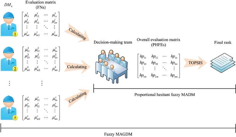
A novel approach for fuzzy MAGDM.
6.2. Numerical example
In practice, in order to evaluate the cost-performance of a product, we should first consider how much “performance” it has. Figure 2 shows some keywords and their frequencies of customer reviews for a smart-phone sold in Best Buy.48 Up to March 14, 2016, there are 469 reviews and keyword “screen” appeared 90 times. According to Figure 2, the main factors that involve in the customer reviews and affect the performance of a smart-phone can be summarized as follows: C1: system optimization, C2: appearance and system UI design, and C3: hardware configuration. Consider a problem that a decision-making team consisted of five decision makers DMk(k = 1,2,…,5) is invited to evaluate the performance of four smart-phones Ai(i = 1,2,…,4). Using FNs, five evaluation matrices are provided as follows.

Customer reviews for a smart-phone.
To solve this problem, we conduct the MAGDM approach proposed in Subsection 4.1 as follows:
Step 1. Based on the evaluation matrices Uk(k = 1,2,…,5), the overall evaluation matrix is U = [phij]4×3, where
Step 2. Following Definition 12, the values of the score and deviation functions for the elements in the overall evaluation matrix U are shown in Table 2.
Step 3. Because all attributes are benefit attributes, based on Definition 13, the positive ideal solution is
and the negative ideal solution isStep 4. Based on Definition 11, the separations of each alternative from the PIS are
Step 5. The closeness coefficients of each alternative with respect to the ideal solutions are Coef1 = 0.8037, Coef2 = 0.5698, Coef3 = 0.4514, Coef4 = 0.4141.
Step 6. The ranking order of all smart-phones on the performance is A1 ≻ A2 ≻ A3 ≻ A4.
| C1 | C2 | C3 | |||||||
|---|---|---|---|---|---|---|---|---|---|
| Score | Deviation | Rank | Score | Deviation | Rank | Score | Deviation | Rank | |
| A1 | 0.420 | 0.107 | 3 | 0.466 | 0.037 | 1 | 0.632 | 0.038 | 1 |
| A2 | 0.530 | 0.022 | 2 | 0.460 | 0.002 | 2 | 0.536 | 0.094 | 2 |
| A3 | 0.650 | 0.070 | 1 | 0.372 | 0.001 | 3 | 0.140 | 0.000 | 4 |
| A4 | 0.270 | 0.007 | 4 | 0.280 | 0.014 | 4 | 0.522 | 0.017 | 3 |
Values of score and deviation functions for elements in matrix U
Therefore, Smart-phone A1 possesses the best performance. This is because A1 not only contains a relatively perfect appearance and system UI design, but also has the best hardware configuration (see Table 1). Although the producer of A3 is not good at the appearance and system UI design, he does the best job in the system optimization with the worst hardware configuration. Consequently, the manufacturer of A1 may consider cooperating with the producer of A3 on the system optimization.
Under the system optimization (C1), ph41 = {(0.37,0.20), (0.32,0.40), (0.17,0.40)} indicates that all decision makers think the evaluation value for Smart-phone A4 is no more than 0.37, and ph31 = {(0.81,0.60), (0.69,0.20), (0.13,0.20)} represents that 60% decision makers think that for Smart-phone A3 is 0.81. Therefore, A3 is better than A4 under attribute C1. Because the producer of A3 does the best job in this attribute, PHFE ph31 then is the positive ideal value under the system optimization. Similarly, PHFEs ph12 and ph13 are the positive ideal values with respect to attributes C2 and C3, which is the key factor that contributes to A1 having the shortest distance from the PIS.
According to the concept of TOPSIS, the higher rank indicates that an alternative is closer to PIS and farther from NIS simultaneously. Smart-phone A2 appears better than A3 and A4 because of the farthest distance from the NIS (i.e.,
7. Comparison
The proposed PHFSs incorporates the proportional information into HFSs, this section is devoted to clarifying the necessity of our conceptual extension in this paper by providing a comparison between the proportional hesitant fuzzy TOPSIS approach and the hesitant fuzzy TOPSIS approach.
7.1. Hesitant fuzzy TOPSIS approach for MAGDM
Ignoring the proportional information, the main steps of the hesitant fuzzy TOPSIS approach for the MAGDM are:
Step 1′. Decision makers DMk(k ∈ S) provide evaluation matrices
Step 2′. Calculate the overall evaluation information. The overall evaluation matrix is represented as U′ = [hij]m×n, where hij(i ∈ M, j ∈ N) is a HFE.
The fuzzy MAGDM is therefore converted into the hesitant fuzzy MADM, which can be solved by utilizing the hesitant fuzzy TOPSIS approach proposed by Xu and Zhang37, however, we use the hesitant normalized Hamming distance to measure the distance between HFEs.
Similar to the proportional hesitant fuzzy TOPSIS approach proposed in Subsection 4.1, the hesitant fuzzy TOPSIS approach can objectively solve the fuzzy MAGDM problem with having a clear understanding on whether an alternative is good at or bad in some attributes. Transforming the fuzzy MAGDM into the hesitant fuzzy MADM may also reduce the complexity of the decision-making system. However, the proportional information (or the preferences of the decision-making team) is not considered into the decision process.
7.2. Dealing with numerical example in Subsection 4.2 through hesitant fuzzy TOPSIS approach
Based on hesitant fuzzy TOPSIS approach, the numerical example in Subsection 4.2 can be similarly solved as follows:
Step 1′. According to the evaluation matrices Uk(k = 1,2,…,5), the overall evaluation matrix is U′ = [hij]4×3, where
h11 = {0.82,0.17,0.12},
h12 = {0.67,0.65,0.53,0.26,0.22},
h13 = {0.73,0.24},
h21 = {0.65,0.35},
h22 = {0.54,0.44},
h23 = {0.98,0.76,0.53,0.23,0.18},
h31 = {0.81,0.69,0.13},
h32 = {0.42,0.36},
h33 = {0.14},
h41 = {0.37,0.32,0.17},
h42 = {0.46,0.32,0.15},
h43 = {0.63,0.36}.
Step 2′. Following Definition 3, the score function values for the elements in the overall evaluation matrix U′ are shown in Table 3.
Step 3′. Based on Definition 4, the positive ideal solution is U′+ = {h31, h22, h23}, and the negative ideal solution is U′− = {h41, h42, h33}.
Step 4′. Suppose the decision makers are all pessimistic. Following Definition 5, the separations of each alternative from the PIS are S′1+= 0.1907, S′2+= 0.0800, S′3+= 0.1653, S′4+ = 0.2309, and the separations of each alternative from the NIS are S′1− = 0.2606, S′2− = 0.2409, S′3− = 0.1267, S′4− = 0.1183.
Step 5′. The closeness coefficients of each alternative with respect to the ideal solutions are Coef′1 = 0.5774, Coef′2 = 0.7507, Coef′3 = 0.4338, Coef′4 = 0.3388.
Step 6′. The ranking order using the hesitant fuzzy TOPSIS approach then is A2 ≻ A1 ≻ A3 ≻ A4.
| C1 | C2 | C3 | ||||
|---|---|---|---|---|---|---|
| Score | Rank | Score | Rank | Score | Rank | |
| A1 | 0.370 | 3 | 0.466 | 2 | 0.485 | 3 |
| A2 | 0.500 | 2 | 0.490 | 1 | 0.536 | 1 |
| A3 | 0.543 | 1 | 0.390 | 3 | 0.140 | 4 |
| A4 | 0.287 | 4 | 0.310 | 4 | 0.495 | 2 |
Values of score function for elements inU′
7.3. Discussion
The ranking order of all alternatives obtained by the hesitant fuzzy TOPSIS approach is A2 ≻ A1 ≻ A3 ≻ A4, whereas it is A1 ≻ A2 ≻ A3 A4 gained by the proportional hesitant fuzzy TOPSIS approach proposed in Subsection 4.1. The difference is the ranking order between A1 and A2, i.e., A2 ≻ A1 for the former while A1 ≻ A2 for the latter. The main reason is that the proportional hesitant fuzzy TOPSIS approach considers both the membership degrees and their associated proportions into the decision process, whereas the hesitant fuzzy TOPSIS approach only focuses on the membership degrees but ignores the proportional information. Comparing with the latter, the proportional hesitant fuzzy TOPSIS approach has the following advantages:
- (1)
Ignoring the proportions may lead to inaccurate average evaluation values for the hesitant fuzzy information. For example, ph13 = {(0.73,0.80),(0.24,0.20)} indicates that most of the decision makers provide a relatively good evaluation for alternative A1 under attribute C3. Then, the average evaluation value of it should be more than 0.73×0.8 = 0.584, which is larger than sHFE(h23) = s(ph23) = 0.536. However, under attribute C3, the average evaluation value of A1 is less than that of A2 by utilizing the hesitant fuzzy TOPSIS approach (see Table 2). Therefore, considering the proportional information in the proportional hesitant fuzzy TOPSIS approach may improve the rationality of the positive/negative ideal solution.
- (2)
In terms of the distance measure, as mentioned in Subsection 3.1, the processes (i.e., “ordering” and “adding”) without changing the average evaluation value in each PHFE are beneficial to obtain a relatively accurate distance measure. Therefore, the proportional hesitant fuzzy TOPSIS approach may contribute to more accurate separations of each alternative from the PIS/NIS.
- (3)
For the proportional information ignored in the hesitant fuzzy TOPSIS approach, the proportional hesitant fuzzy TOPSIS approach regards it as the preferences of the decision-making team, which may increase the reliability of the decision result.
8. Conclusions
In this paper, in view of past studies cannot reasonably model a practical case in which a team could not reach agreement on a fuzzy decision, and the proportions of the membership degrees are measurable, the concept of PHFSs has been proposed. As the component of PHFSs, PHFEs contain two aspects of information: the possible membership values and their associated proportions. Because the proportions represent the preferences of the decision-making team, the PHFSs appear more accurate and reasonable than HFSs to model the uncertainty produced by human being’s doubt. According to Rodríguez et al.,4 the main advantages of PHFSs and their operations are summarized as follows.
- (1)
Following the Fundamental Principle of a Generalization4, the PHFS is not only a mathematic extension of the HFS, but also a more accurate representation of people’s hesitancy in stating their preferences over objects. The novel representation has a large number of applications in practice.
- (2)
The repeated values in decision making problem are usually removed within HFSs, whereas PHFSs convert them into the proportions, which also may decrease the degree of the hesitancy.
- (3)
In terms of the distance measure on PHFSs, the ordering method on the basis of both the membership degree and its associated proportion may contribute to reasonable orders of the elements in PHFEs. For the adding method, any addition does not change the distance measure value between two PHFEs.
Besides, a novel MAGDM approach for the fuzzy information has also been developed in this paper. First, the fuzzy MAGDM (expressed by classical FNs) is converted into the proportional hesitant fuzzy MADM (expressed by PHFEs) by calculating the proportions of the associated membership degrees. After that, the alternatives are ranked by the proportional hesitant fuzzy TOPSIS approach. This proposal is different from the traditional fuzzy MAGDM approach, in which the evaluation values are always represented by the FNs as shown in Stage 1 of Section 4. A numerical example is provided to illustrate the fuzzy multiple attribute group decision making process.
As future work, we consider the study of the related operations and properties on PHFSs according to HFSs. Especially, the union and intersection operations on PHFEs in this paper are defined from the angle of probability with the assumption that all PHFEs are mutually independent (see Definition 9). Therefore, defining such operations without that assumption or on the basis of the t-norms and t-conorms49 could be a fruitful research of our work.
Acknowledgments
This work was supported by the Theme-based Research Projects of the Research Grants Council (Grant no. T32-101/15-R) and partly supported by the Key Project of the National Natural Science Foundation of China (Grant No. 71231007) the National Natural Science Foundation of China (Grant No. 71373222) and the CAAC Scientific Research Base on Aviation Flight Technology and Safety (Grant No. F2015KF01).
Footnotes
This paper in part is inspired by the rapid development of semantics for evaluation information as we have briefly introduced here.
In fact, PHFSs can as well be utilized to characterize the proportional hesitant information derived from the “time” dimension, which can be generated from a dynamic evaluation process conducted by a single decision maker. The information representation construction in this paper, however, focuses on the manifestation of group evaluations, therefore, we place restrictions on our discussion to the management of proportional hesitant group decision making resulting from the “space” dimension. Application of PHFSs in the modelling of individual evaluations is not discussed at the current stage to keep the paper stay focused, and we would like to leave it for future investigation, mainly because this issue does not jeopardize methodological integrity or pose any theoretical barriers for comprehension.
References
Cite this article
TY  - JOUR
AU  - Sheng-Hua Xiong
AU  - Zhen-Song Chen
AU  - Kwai-Sang Chin
PY  - 2018
DA  - 2018/01/01
TI  - A Novel MAGDM Approach With Proportional Hesitant Fuzzy Sets
JO  - International Journal of Computational Intelligence Systems
SP  - 256
EP  - 271
VL  - 11
IS  - 1
SN  - 1875-6883
UR  - https://doi.org/10.2991/ijcis.11.1.20
DO  - 10.2991/ijcis.11.1.20
ID  - Xiong2018
ER  -