
An Optimal Task-Scheduling Strategy for Large-Scale Astronomical Workloads using In-transit Computation Model
- DOI
- 10.2991/ijcis.11.1.45How to use a DOI?
- Keywords
- Task Scheduling; In-transit Computation; Load Distribution; Fog Computing; Genetic Algorithm
- Abstract
The Sloan Digital Sky Survey (SDSS) has been one of the most successful sky surveys in the history of astronomy. To map the universe, SDSS uses their telescopes to take pictures of the sky over the whole survey area. Now the total SDSS data volume is larger than 125 TB since every night telescopes produce about 200 GB of data. To improve the processing efficiency of such large-scale astronomical data, we develop an optimal task-scheduling strategy by using in-transit computation model under fog computing. Within the proposed strategy, we design a global optimization technique to derive an optimal load distribution among heterogeneously computational resources. Finally, we conduct various experiments to illustrate the correctness and effectiveness of the proposed strategy. Experimental results show that it can significantly decrease the processing time of large-scale workloads.
- Copyright
- © 2018, the Authors. Published by Atlantis Press.
- Open Access
- This is an open access article under the CC BY-NC license (http://creativecommons.org/licences/by-nc/4.0/).
1. Introduction
For millennia, twinkling stars in the night sky have always inspired our curiosity about the universe. Astronomers have launched various scientific sky surveys in the last century attempting to map the universe, over ever-larger areas, to ever-greater depths, and over an ever-increasing range of wavelengths. Among these surveys, the Sloan Digital Sky Survey (SDSS)1 has created the most detailed three-dimensional maps of the universe ever made, with deep multi-color images of more than one third of the entire night sky, and spectra for more than three million astronomical objects.
SDSS has progressed through several phases. In its first five years of operations, SDSS-I (2000–2005) carried out deep multicolor imaging over 8000 square degrees and measured spectra of more than 700,000 objects. With an ever-growing collaboration, SDSS-II (2005–2008) completed the goals of imaging half the northern sky and mapping the 3-dimensional clustering of one million galaxies and 100,000 quasars. SDSS-III (2008–2014) undertook a major upgrade of the venerable spectrographs2. In July 2014, SDSS-IV was launched. It is an extensive imaging and spectroscopic survey of the Northern and Southern sky, using a dedicated 2.5-meter telescope located at southeast New Mexico and the du Pont Telescope at northern Chile2. Each telescope is fixed to point directly up at the sky and images a “stripe” of the sky over the course of night. As the Earth rotates, more of the sky becomes visible above the telescopes. Every night the telescopes produce about 200 GB of data. Now the total SDSS data volume is larger than 125 TB2.
Each image taken by telescopes is composed of myriad pixels, each pixel of which captures the brightness of every tiny point in the sky. But the sky is not made of pixels. Data managers for SDSS requires to extract digitized data from images and process the extracted data to produce information they can use to identify and measure properties of stars and galaxies. It is worth noting that scientists must handle the astronomical workloads as quickly as possible because SDSS astronomers need the information to configure their telescope to work most efficiently during the next dark phase of the moon. If too much time goes by, we might miss the immediate next season of the target objects.
Such large-scale astronomical data could not be processed efficiently without network-based computing systems. One of the key issues in networked computation is obtaining an optimal scheduling strategy, including partition and distribution of workload among computational resources, to achieve shortest processing time. An optimal scheduling strategy depends mainly on the network architecture as well as the number of computational resources and their computing capabilities. Mani and Ghose3 studied the distribution of divisible workload in a homogeneous linear network and derived recursive equations for obtaining an optimal load partition. Later, asymptotic solutions for homogeneous bus networks were obtained 4. For heterogeneous star networks, Bharadwaj et al.5 derived a closed-form expression for an optimal load partition to achieve shortest processing time. The task-scheduling problem turns out to be more difficult when practical issues like the computation and communication start-up overheads are considered. Carroll6 and Ghanbari7 studied optimal scheduling strategies for bus and tree networks with arbitrary start-up overheads, respectively. Later on, similar studies have been made on a variety of distributed networks, such as Gaussian, mesh, torus networks8, complete b-Ary tree networks9, heterogeneous clusters10, and cloud computing systems11.
It should be noted that even the most advanced cloud computing architecture still faces challenge to handle a large amount of astronomical data. Fog Computing is becoming widely known as being the one that extends cloud computing to edge devices and processes directly on the edge devices, thus minimizing the amount of data that is transferred to the cloud12. One ubiquitous edge device is network data center. Compared to data centers hosted by cloud providers, network data centers are managed and operated by network providers, which constitute an important part of the current Internet infrastructure. Fog computing can exploit network data centers along the path when workloads are in transit from the user side to cloud data center, so that the spare compute capacities of network data centers could be utilized more efficiently and the processing time of workloads shall be decreased simultaneously. With this idea in mind, Zou et al.13,14 proposed an in-transit computation infrastructure composed of an ensemble of computational resources, inclusive of a cloud data center and a certain amount of network data centers connecting the source (user) and destination (cloud data center). We employ this in-transit computation model in this work to improve the processing efficiency of astronomical workloads. Our main objective is deriving an optimal task-scheduling strategy for in-transit computation under fog computing so that the processing time of large-scale workloads could be minimized.
The remaining of this paper is organized as follows. Section 2 establishes a novel task-scheduling model for in-transit computation. To solve this model, we accordingly design an effective genetic algorithm in Section 3, which will be evaluated through experiments in Section 4. In the last section, conclusions are obtainable.
2. In-transit Computation under Fog Computing
In this section, we shall first formally define the task-scheduling problem we address and introduce all the notations and definitions used throughout this paper. Then we propose a novel task-scheduling model for in-transit computation of large-scale workloads under for computing.
2.1. Problem Description
Suppose that an astronomer needs to compute a workload Wtotal, for example searching among astronomical database or analyzing astronomical data for a certain purpose. The location where workload stores is defined as source s, while the remote cloud data center is defined as destination d. Workload Wtotal transfers from source s to destination d through a network path composed of n in-transit network data centers {f1, f2, ⋯ , fn} as illustrated in Fig.1. Now the problem lies in how to take full advantage of in-transit computation by deriving an optimal load distribution strategy among (n + 1) fog nodes, including n in-transit network data centers and the cloud data center, also denoted as fn+1.
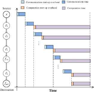
Timing diagram for in-transit computation
Note that astronomical data, although large in size, are generally partitionable, meaning that they can be partitioned into any number of fractions, or at least fine-grained fractions, and that there are no precedence relationships among these fractions so that they can be independently processed on distributed compute platforms. Hence, workload Wtotal will be partitioned into (n + 1) fractions and processed by (n+1) fog nodes independently. Note that source s does not participate in workload computation. We can observe from Fig.1 that after receiving the whole workload from resource s, fog node f1, an in-transit network data center, keeps a fraction α1 of Wtotal for itself and transmits the remaining (Wtotal − α1) to its right immediate neighbor f2. Similarly, fog node fi keeps a fraction αi of Wtotal for itself and transmits the remaining
Source s is assumed to start distributing the whole package of workload Wtotal to fog node f1 at time t = 0. It takes node fi time
Let Pi denote the time when node fi finishes transmitting load fractions to node fi+1. We have
Finally, we can obtain the processing time T of the total workload as T = max{T1,T2, ⋯, Tn+1}.
2.2. In-transit Computation Model
Here we formulate a new in-transit computation model under fog computing.
- (1)
A = {α1, ⋯, αn+1};
- (2)
Ti = Pi + ci + wiαi with i = 1, 2, ⋯, n + 1;
- (3)
P1 = o0 + z0Wtotal + o1 + z1(Wtotal − α1);
- (4)
- (5)
Pn+1 = Pn.
- (i)
αi ∈ A, 0 < αi < Wtotal, i = 1, 2, ⋯, n + 1;
- (ii)
There are (n + 1) variables involved in this model. Constraints (i) and (ii) indicate that load fractions assigned on fog nodes should be nonnegative and not larger than the entire workload, and that the sum of all load fractions equals the entire workload.
3. Optimal Task-Scheduling Strategy
In this section, we shall design a Genetic Algorithm (GA) searching for an optimal load partition A = {α1, α2, ⋯, αn+1} for the proposed in-transit computation model. We select GAs to solve our model because GAs have been proven to be a promising technique for combinatorial optimization problems, especially for task-scheduling problems.
3.1. Encoding and Genetic Operators
The key point of finding an optimal solution by using GAs is to develop an encoding scheme that can represent the problem to be solved directly while satisfying the problem constraints easily. In this paper, an individual is real coded directly as I = (α1, α2, ⋯, αn+1). For a given individual I, if ∃i, αi⩽0 or
As a simple example, assume that there are n = 6 fog nodes in the system, inclusive of 5 in-transit network data centers along the path from source to destination (cloud data center). The size of the entire workload is 1000 units. A possible encoding scheme is given as follows:
We observe that ∀i, αi > 0 and
According to our proposed in-transit computation model, we have a special constraint as
We adopt two-point mutation on offsprings generated by crossover according to a user-definable mutation probability. This probability should be set low; otherwise, the search will turn into a primitive random search. In detail, we randomly generate two integers p and q satisfying that 1 ⩽p < q ⩽(n + 1), then exchanging genes αp and αq of individual I. It can be expected that offsprings generated by this mutation operator satisfy all of the constraints in our proposed model by default.
3.2. Local Search
To accelerate the convergence of the proposed GA, we introduce a local search operator in this paper. The main idea is to transfer proper size of load from the fog node with the longest processing time Tmax to the one with the shortest processing time Tmin, so that all of the fog nodes will eventually stop computing at the same time instant. The process of the local search operator is given as follows.
- Step 1
For a given individual I = (α1, α2, ⋯ , αn+1), let P0 = o0 + z0 Wtotal.
- Step 2
FOR (i = 1,2,⋯ , n)
Let
ENDFOR
- Step 3
Let Tn+1 = Pn + cn+1 + wn+1αn+1.
- Step 4
Among all fog nodes {f1, f2, ⋯ , fn+1}, find node fmax with the longest processing time Tmax and fog node fmin with the shortest processing time Tmin. Calculate their time difference by ∆ = Tmax − Tmin.
- Step 5
Let β = ∆/max{zmax, zmin}. Update individual I by αmax = αmax − β and αmin = αmin + β.
Figure 2 shows a timing diagram that corresponds to an individual before applying local search. As illustrated in Fig. 2, node f1 has the longest processing time T1 and f3 has the shortest processing time T3. Thus fmax = f1 and fmin = f3. After load balancing between f1 and f3 by local search operator, a possible timing diagram is shown in Fig. 3. It can be observed that the time difference between T1 and T3 illustrated in Fig. 3 becomes much smaller than that in Fig.2. Hence, the total processing time of the entire workload would be decreased.
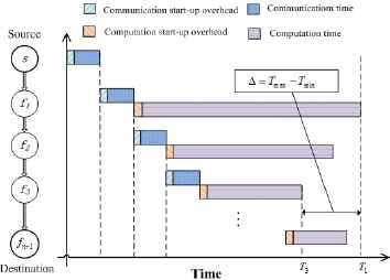
Timing diagram before applying local search
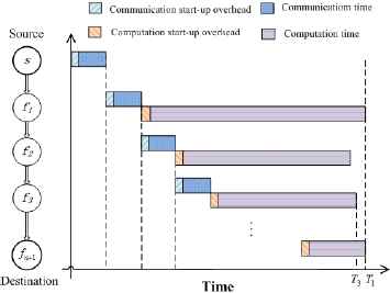
Timing diagram after applying local search
3.3. Framework of the Proposed Algorithm
Once encoding scheme is defined, a GA initializes a population of individuals and then improves them through repetitive applications of genetic operators, including crossover, mutation, local search, and selection. Given workload Wtotal, population size Popsize, crossover probability pcros, mutation probability pmut, elitist number E = 5, and stop criterion, the framework of our proposed GA is given as follows.
- Step 1
(Initialization) Randomly generate Popsize individuals as initial population Pop(0) according to the encoding scheme. For each I ∈ Pop(0), compute processing time T of workload Wtotal and take 1/T as the fitness value of I. Let generation number t = 0.
- Step 2
(Crossover) Select Popsize individuals into the crossover pool from Pop(t) by roulette wheel selection. Apply two-point crossover on each pair of parents selected from the crossover pool according to pcros and then normalize the newly generated offsprings to ensure that
- Step 3
(Mutation) Apply two-point mutation on each of the selected individuals from O1(t) according to pmut. All newly generated off-springs constitute a set denoted by O2(t).
- Step 4
(Local Search) Apply local search operator on each individual in set O1(t) ∪ O2(t).
- Step 5
(Selection) Select the best E individuals for the next population Pop(t + 1) from set Pop(t) ∪ O1(t) ∪ O2(t). Select the remaining Popsize − E individuals for Pop(t + 1) by roulette wheel selection also from set Pop(t) ∪ O1(t) ∪ O2(t). Let t = t + 1.
- Step 6
(Stopping Criteria) If a fixed number of generations reached, then stop and return the best individual I in the current population; otherwise, go to Step 2.
4. Experimental Results and Analysis
As we mentioned earlier, every night the telescopes of SDSS, including the primary 2.5m telescope, 0.5m photometric telescope, and 10 micron all sky scanner, produce about 200 GB of raw imaging data. In our simulation, we have considered this actual data size and normalized it into 10000 units. Then a series of operators are required to process these large-scale telescope imaging data under fog computing, ultimately producing a variety of products including images with instrumental signatures removed, a photometric solution for the night, and a catalog of objects found in the data. The computation speed of each fog node processing every unit of astronomical data is recorded in Table 1.
| pi | oi | ci | zi | wi | pi | oi | ci | zi | wi | pi | oi | ci | zi | wi |
|---|---|---|---|---|---|---|---|---|---|---|---|---|---|---|
| p1 | 5.40 | 9.87 | 0.14 | 29.71 | p8 | 5.03 | 2.21 | 0.14 | 37.26 | p15 | 7.00 | 6.48 | 0.20 | 32.62 |
| p2 | 6.97 | 1.40 | 0.19 | 30.52 | p9 | 3.06 | 4.18 | 0.15 | 24.33 | p16 | 9.40 | 6.84 | 0.12 | 21.28 |
| p3 | 7.22 | 6.96 | 0.19 | 39.53 | p10 | 4.03 | 6.49 | 0.19 | 36.73 | p17 | 2.07 | 7.30 | 0.20 | 35.44 |
| p4 | 6.50 | 2.50 | 0.17 | 20.51 | p11 | 1.63 | 3.39 | 0.11 | 27.39 | p18 | 8.80 | 4.40 | 0.18 | 33.42 |
| p5 | 2.34 | 3.38 | 0.13 | 30.63 | p12 | 9.30 | 4.34 | 0.12 | 30.37 | p19 | 7.93 | 8.12 | 0.17 | 34.67 |
| p6 | 4.23 | 9.35 | 0.12 | 33.70 | p13 | 3.59 | 9.05 | 0.14 | 39.52 | p20 | 2.46 | 9.28 | 0.16 | 0.30 |
| p7 | 9.71 | 3.14 | 0.16 | 36.62 | p14 | 1.39 | 7.68 | 0.15 | 30.99 | — | — | — | — | — |
Parameters for fog nodes
In each run of our proposed GA, the following parameters are set: Popsize = 100, crossover probability pcros = 0.8, mutation probability pmut = 0.02, elitist number E = 5, and stop criterion t = 2500.
4.1. Correctness Evaluation
We conduct two experiments to validate the correctness of our proposed GA. In each experiment, we employ a fog computing system with 20 fog nodes, including 19 in-transit network data centers and one cloud data center. In the first experiment, we fix system parameters as given in Table 1 and vary the workload size from 500 to 2500 units. Figs. 4 and 5 collect the experimental resutls. In the second experiment, we fix workload size as Wtotal = 1000 unites and vary the network scenarios where the compute capability of cloud data center is q times more powerful than that of in-transit fog nodes, where q ∈ {5, 10, 15, 20, 25}. Figs. 6 and 7 record the results.
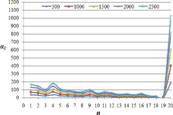
Optimal load partitions for different workloads
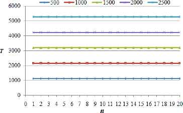
Finish times of fog nodes for different workloads
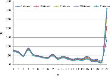
Optimal load partitions under different networks
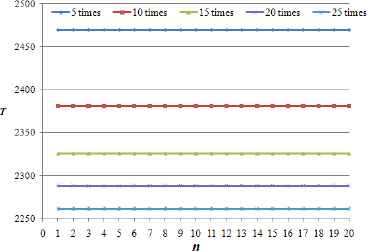
Finish times of fog nodes under different networks
We observe from Figs.5 and 7 that all fog nodes stop computing at the same time for every test. Hence, the proposed algorithm can obtain an optimal task-scheduling strategy that achieves minimum processing time. As expected, we can see from Figs.4 and 6 that the load fraction assigned to the last node is much larger than that assigned to other fog nodes because the last node represents a cloud data center with high-performance capability, while the other nodes are in-transit network data centers with relatively low-performance capabilities.
4.2. Performance Evaluation
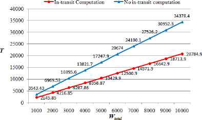
To evaluate the effectiveness of the proposed algorithm, we make two comparisons between our algorithm, labeled as “In-transit computation” in the experiment results, and the task-scheduling strategy with only cloud data center performing computation, labeled as “No In-transit computation.” Figure 8 records the comparison results obtained for different workloads ranging from 1000 to 10000 units, while Fig. 9 collects the experimental results obtained under different network scenarios with network size varying from 10 to 30.
Comparison between in-transit computation and no in-transit computation for different workloads
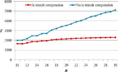
Comparison between in-transit computation and no in-transit computation under different network scenarios
It can be observed from Figs.8 and 9 that the processing time obtained by “In-transit computation” strategy is much less than that by “No in-transit computation” strategy for each test, and that the time difference between them grows with increasing workload size and network size. As shown in Fig.8, when workload size is as large as 10000 units in our experiment, the processing time obtained by the “In-transit computation” strategy shows a gain of 65.4% compared to “No In-transit computation” strategy. Also, it can be seen from Fig.9 that when there are 30 fog nodes in the network system, the “In-transit computation” strategy reduces the processing time by over 55.3% compared to “No Intransit computation” strategy. Therefore, it is clear that our proposed algorithm for in-transit computation can derive an optimal task-scheduling strategy that significantly decreases the processing time of large-scale workloads. This holds even in cases where in-transit fog nodes are not very powerful in computation compared to the cloud data center.
5. Conclusions
In this paper, we have addressed the task-scheduling problem for in-transit computation of large-scale astronomical workloads under fog computing. We built a novel task-scheduling model and proposed a genetic algorithm to derive an optimal load distribution strategy. We have explicitly considered the astronomical imaging data taken by telescopes of SDSS as our reference size of data volume in our extensive experiments. We demonstrated that the proposed algorithm could significantly decrease the processing time of large-scale workloads by intransit computation. An important and immediate useful extension to the study posed in this paper is considering complex networks with more than one network path available from source to destination, and deriving an optimal task-scheduling strategy, including selection of in-transit nodes along the path and distribution of workloads among them.
Acknowledgments
This work was initiated and conducted jointly when the second author visited Department of CS, Cardiff University, in September 2016, and supported by MOE Tier-1 grant No. R-263-000-C14-112. This study on data distribution aspects serves as a preliminary study for possible extensions to take care of security aspects while designing IOT based platforms to handle large-scale data processing for intelligent transportation system in Singapore. The first author would like to acknowledge the funding supported by National Natural Science Foundation of China (No.61402350, No.61472297, and No.61572391).
References
Cite this article
TY  - JOUR
AU  - Xiaoli Wang
AU  - Bharadwaj Veeravalli
AU  - Omer F. Rana
PY  - 2018
DA  - 2018/01/22
TI  - An Optimal Task-Scheduling Strategy for Large-Scale Astronomical Workloads using In-transit Computation Model
JO  - International Journal of Computational Intelligence Systems
SP  - 600
EP  - 607
VL  - 11
IS  - 1
SN  - 1875-6883
UR  - https://doi.org/10.2991/ijcis.11.1.45
DO  - 10.2991/ijcis.11.1.45
ID  - Wang2018
ER  -