
Machine Learning for Stellar Magnetic Field Determination
- DOI
- 10.2991/ijcis.11.1.46How to use a DOI?
- Keywords
- Artificial Neural Networks; Machine Learning; Stellar: Magnetic Fields; Parameter Determination
- Abstract
Abstract
In this work we present the results for the automatic determination of the mean longitudinal magnetic field in polarized stellar spectra through the analysis of spectropolarimetric observations. In order to determine this important parameter, we first developed a synthetic database encompassing a set of different stellar spectra, each one defined by a set of free parameters. Then, we used supervised learning for artificial neural networks, a machine learning approach, to achieve our goal.
- Copyright
- © 2018, the Authors. Published by Atlantis Press.
- Open Access
- This is an open access article under the CC BY-NC license (http://creativecommons.org/licences/by-nc/4.0/).
1. Introduction
Nowadays there are plenty of astronomical databases available,1,2,3,4 containing enormous quantities of data, both real and synthetic. Hence, analysis and automatic extraction of relevant information from these collections have become an important task. Although there have been some successful efforts to retrieve some parameters from these databases,5,6,7 magnetic fields are a particularly complex phenomena and since they cannot be directly measured, their accurate determination is remarkably difficult.8 As a rule of thumb, magnetic fields are measured via the effects of their presence on other observable properties. The most successful method used to detect magnetic fields relies on the Zeeman effect.9 This effect is, essentially, the splitting of a spectral line due to the distortion of electron orbitals as a result of the presence of a magnetic field. This distortion depends on the quantum numbers of the energy level and the magnetic field intensity.10 On a spectrum formed in a region permeated by a magnetic field, the orbital energies between transitions are disturbed and, therefore, the absorption or emission lines might be affected.
The energy for each level is affected by the presence of a magnetic field, and each energy level with quantum number J splits into (2J + 1) states of energy with different magnetic quantum numbers M. The difference between successive energy states (ΔE) is proportional to the magnetic field and to the Landé factor (g), which is a function of the orbital angular momentum (L) and the electron spin (S) as described in Eq. (1).
Energy shifts are given by:
Where μB is the Bohr magneton, B is the magnetic field strength, and M ranges from −J to J, hence the previously mentioned (2J + 1) different states. In the absence of a magnetic field, a transition between two levels, E1 and E2, with Landé factors g1 and g2 is characterized by a single energy level: E2 − E1, but when a magnetic field is applied, the spectral line splits into closely dispersed segments with energies shifted from the original energy by:
Considering Δg = g2 − g1 and ΔM = M2 − M1 we can transform Eq. (3) as:
A dipole transition between levels adheres to the selection rule ΔM = − 1,0,1 and therefore, the resulting spectral lines assemble into three groups; lines due to transitions with ΔM = 0, known as π components and the groups of lines formed by transitions where ΔM = ±1. The latter are known as σ+ when lines are shifted to the right side in wavelength (red shifted) and σ−, when they are blue shifted. Normally, both π and σ groups have several components, and when these components overlap, e.g. when g2 = g1, the transition is called a Zeeman triplet. There are also some cases where lines show no splitting, e.g. when g1 = 0 and J2 = 0, known as magnetic null lines. Each group is characterized by different polarization states11 and their observed intensity depends on the angle between the line of sight and the magnetic field, among other parameters. Therefore, the measurement of the intensity at different polarized states is crucial for the proper characterization of a magnetic field.
The Stokes parameters12 is a widely used representation of polarized states. These parameters are a set of four values, named Stokes I,Q,U and V, that describe the polarization state of electromagnetic radiation11 as follows; Stokes I is the integrated (non polarized) light, Stokes Q and U measure the two directions of linear polarization, and Stokes V measures circular polarization. These parameters are useful in astronomy because both circular and linear polarization states can be measured through appropriate instruments such as polarimeters and spectropolarimeters.
Observations from Stokes I can be used to infer the magnetic field strength if for any given line, we can observe and measure the Zeeman splitting between the π and σ components of the transition. However, other broadening effects -as those induced by rotation, pressure, temperature, and others-can mask the split of the Zeeman components.8 As a result, this technique is useful to measure only very strong magnetic fields, in the order of 103 Gauss (kG) and higher,13 and becomes impractical for weaker fields. To illustrate this, the comparison between two Stokes I spectra for an object simulated with two different values of the effective magnetic field (Heff), 1G and 10G, is shown in Fig. 1. It is clear that the difference between both spectra is practically indistinguishable, emphasizing the complexity of the magnetic field measurements using only the Stokes I parameter.
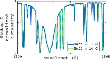
Fragment of the spectra of the Stokes I parameter for a synthetic object simulated with different magnetic field.
Observations from the rest of the Stokes parameters (Q,U and V) are important because they are more sensitive to weaker fields due to the lower influence of other, non-magnetic effects. However, linear polarization produced by magnetic fields is generally weak, so its measurement in stars (associated with Stokes Q and U) is not common.8 Therefore, magnetic field measurements are typically performed using only Stokes I and Stokes V parameters. The Stokes V spectra of the same object depicted in Fig. 1 is shown in Fig. 2. It is clear that the difference between the two cases (1G and 10G) becomes more evident using this parameter.
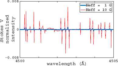
Fragment of the spectra of the Stokes V parameter for a synthetic object simulated with different Heff.
Although the use of Stokes V allows to measure the magnetic field, it is known that, particularly on solar-type stars, magnetic fields are commonly found in the order of 10G,14 at which level the normalized intensity of this parameter is below the noise level. Looking to overcome this problem, several “multi-line” techniques have been developed. These techniques receive their name from the fact that they perform the addition of multiple individual lines on velocity domain,15 resulting in a mean profile or signature, known as multi-Zeeman Signatures (MZS). They encompass all the information from the polarized spectra, decreasing the noise level and at the same time performing a dimensionality data reduction. The most popular of these techniques is the Least Square Deconvolution (LSD) proposed by Donati et al. in Ref. 16, used to measure magnetic fields in several research papers.17,18,19,20
Nonetheless, looking to overcome the restrictions on the LSD method (assumptions of similarity between individual polarized circular lines and Weak Field Approximation) a different technique based on Principal Component Analysis (PCA) has been developed. This technique has been numerically validated to increase the Signal to Noise Ratio (SNR) of the MZS.21,22
2. Methods
In order to perform the automatic determination of the mean longitudinal magnetic field (Heff) from polarized stellar spectra, the use of supervised Artificial Neural Networks (ANN) trained with a synthetic database of Multi-Zeeman Signatures (MZS) was proposed.
To create this database, it is necessary to model the Stokes parameters. This implies solving a set of four coupled first-order linear differential equations,23 each one corresponding to a single Stokes parameter. To address the problem that represents the computing needed to solve this system of equations, known as “Polarized Radiative Transfer (PRT) problem”, several codes have been developed.24,25,26
In this work, the use of the COSSAM code was selected. COSSAM stands for ”COdice per la Sintesi Spettrale nelle Atmosfere Magnetiche” or Code for the spectral synthesis in magnetic atmospheres. It was introduced in its latest form by Stift in Ref. 25. This object-oriented parallel code allows to accurately calculate the Stokes parameters for stars in which their magnetic field is represented by a tilted, eccentric dipole on assumed Local Thermodynamic Equilibrium (LTE).27
In order to calculate the Stokes parameters through COSSAM, it is necessary to define the following physical characteristics of the simulated object:
- (i)
Effective temperature (Teff)
- (ii)
Surface gravity (expressed as logg)
- (iii)
Macro-turbulent velocity (Vturb)
- (iv)
Metallicity [M/H]
- (v)
Atomic transitions (taken from VALD: Vienna Atomic Line Database28)
- (vi)
Micro turbulent velocity (ξ)
- (vii)
Inclination angle (i), is the orientation of the rotational axis with respect to the Line Of Sight (LOS)
- (viii)
Orientation of the magnetic axis with respect to the rotation axis (described by the Euler Angles)
- (ix)
Position of the magnetic dipole inside the star (expressed by two coordinates: x1 and x2)
- (x)
Dipole moment (m)
- (xi)
Projected rotational velocity (v sin i)
- (xii)
Rotational phase
- (xiii)
Pulsational velocity and phase
- (xiv)
Spatial Grid
The first four characteristics (Teff, logg, Vturb and metallicity) define the commonly named “atmospheric model”. Although, all the previously listed characteristics affect the behavior of the Heff to some degree,25 as a first step in our research, it was decided to limit the scope of this paper to only the case where all of the parameters are kept constant except for: Teff, logg, Vturb and m.
In order to build the database, first the widely employed Castelli & Kurucz atmospheric models29 were obtained, then the ATLAS12ada30 code was used to transform them into the required format. Each of these models matches a different combination of the previously mentioned characteristics: Teff, logg and Vturb. For spectra synthesis, only solar metallicity was considered. Next, COSSAM was used employing a dipole centered magnetic model31 and keeping the spatial grid reduced to its simplest form: a single point at the center of the star.
To summarize, our database is integrated by varying the previously mentioned characteristics as shown in Table 1. It is significant to notice that the actual number of atmospheric templates (43) differs from the number expected according to Table 1 (5 * 5 * 2 = 50), because some of the Kurucz templates were not available. It is also important to take into account that Heff varies at two different rates: first, from 1 to 20G at a 1G increment (20 steps), and then from 25 to 200G at a 5G increment (36 steps) resulting in 56 steps.
| Characteristic | First Value | Step | Final Value | Total |
|---|---|---|---|---|
| Atmospheric Models | ||||
| Teff | 5000 | 500 | 7000 | 5 |
| log g | 1 | 1 | 5 | 5 |
| Vturb | 0 | - | 2 | 2 |
| Heff | 1 | 1 | 20 | |
| 25 | 5 | 200 | 56 | |
Database characteristic information
The total number of stellar spectra from the combination of all the parameters is 2048 (43 * 56).
It is important to note that all the parameters that define the magnetic geometry were kept constant, and therefore, the data generated with COSSAM consists of Stokes I and V parameters only.
In order to make the spectra in our database closer to real spectra, which always contains noise, different levels of additive white Gaussian noise were incorporated to the Stokes V vectors (5%, 10%, 20% and 30%) of the simulated (clean) spectra. A small fragment of the resulting noisy spectra for each case is shown in Fig. 3. These Noise Percentages (NP) were calculated as:
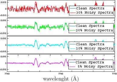
Fragment of the noisy spectra of the Stokes V parameter.
Following this definition and considering that a standard SNR is defined as:
According to Eq. (7), our NP levels turn into SNR as: 400, 100, 25 and
To create the polarized signatures (MZS) from Stokes V, only the first component of PCA was used. The length of the MZS was set to 279 points, ranging from −139 to 139 km/s. Two examples of the resulting MZS are shown in Fig. 4. From this figure, it is evident that most of the information is contained in a smaller range (in this case, between −20 and 20 km/s).
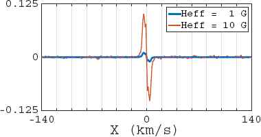
MZS comparison for two synthetic objects with different Heff.
The final database, used to train an ANN to determine Heff, includes 10,240 of these Stokes V signatures, corresponding to both clean and noisy spectra. Stokes I signatures might be useful to determine other parameters (Teff, logg, etc.).
After the evaluation of different architectures, the chosen ANN consists of a fully connected network with just one hidden layer. The input layer has 279 neurons (each one corresponding to a point from the MZS), the hidden layer has 10 neurons and the output layer has one neuron. In order to train the ANN, several training algorithms for the noise-free case were tested. For the noisy case, the algorithm with the best perfomance was chosen to train the final ANN. To validate the performance of each ANN, a k-fold cross validation process39 with k = 5 was performed.
3. Results and Discussion
The mean measures of dispersion from the k-fold cross validation of each ANN using only clean signatures are shown in Table 2; each one of the acronyms for the algorithms (listed on the header) stands for:
- •
bfg: BFGS quasi-Newton Back Propagation (BP)
- •
br : Bayesian regularization
- •
cgb: Powell-Beale Conjugate Gradient (CJ) BP
- •
cgf: Fletcher-Powell CJ BP
- •
cgp: Polak-Ribiere CJ BP
- •
gda: Gradient Descent (GD) with adaptive lr BP
- •
gdx: GD with momentum & adaptive lr BP
- •
lm : Levenberg-Marquardt BP
- •
oss: One Step Secant
- •
rp : Resilient BP
- •
scg: Scaled Conjugate Gradient
| bfg | br | cgb | cgf | cgp | gda | gdx | lm | oss | rp | scg | |
|---|---|---|---|---|---|---|---|---|---|---|---|
| R | 0.9876 | 0.9983 | 0.9982 | 0.9975 | 0.9975 | 0.9818 | 0.9787 | 0.9982 | 0.9972 | 0.9954 | 0.9974 |
| MSE | 101.923 | 13.618 | 15.148 | 20.547 | 20.265 | 150.93 | 175.822 | 13.383 | 23.193 | 37.463 | 21.621 |
| RMSE | 9.9902 | 3.6651 | 3.8898 | 4.5279 | 4.4930 | 12.2596 | 13.1695 | 3.6743 | 4.8031 | 6.0966 | 4.6339 |
| RRSE | 0.1558 | 0.0571 | 0.0606 | 0.0706 | 0.0700 | 0.1912 | 0.2053 | 0.0578 | 0.0749 | 0.0952 | 0.0723 |
| MAE | 5.7469 | 1.8140 | 2.3632 | 2.7658 | 2.6847 | 7.5064 | 7.6297 | 1.7796 | 2.9001 | 3.6230 | 2.7722 |
| RAE | 0.1011 | 0.0319 | 0.0415 | 0.0486 | 0.0471 | 0.1319 | 0.1341 | 0.0312 | 0.0509 | 0.0638 | 0.0487 |
Training Algorithms: Mean Measures of Dispersion
In the case of added noise to the stellar spectra it was decided, based on the measurements from table 2, to use Bayessian Regularization.40 This algorithm has both the best correlation coefficient (R) as well as the best Root Mean Square Error (RMSE).
From here on, all the results shown correspond to the final database (including both noisy and clean spectra). The regression performance for Heff obtained with the ANN is shown in Fig. 5. The Percentage Errors41 (PE) from this regression have a normal distribution with μ = −1.5135% and σ = 7.2836%. The histogram that corresponds to these errors and their respective Probability Distribution Function (PDF); calculated using the normfit function from Matlab R2015a, is shown in Fig. 6. It is important to notice how the calculated PDF (shown as a continuous red line) seems to highly underestimate the real performance of the ANN. This effect is produced by the high percentage errors found for the lowest fields, around 1G. If the PDF is calculated dismissing these errors, i.e. higher than 20%, then a different PDF more faithful to the actual distribution of the histogram can be found. This PDF, with μ = −0.5937% and σ = 3.9310%, is also shown in Fig. 6 as a dashed yellow line. Further statistical measures of the regression performance are shown in Table 3.

Heff Regression plot.
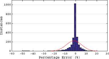
Percentage Errors Histogram and PDF.
| Clean | Noisy 5% | Noisy 10% | Noisy 20% | Noisy 30% | Combined | |
|---|---|---|---|---|---|---|
| R | 1 | 0.9997 | 0.9981 | 0.9957 | 0.9919 | 0.9983 |
| MSE | 0.37x10⁻³ | 2.2525 | 15.4002 | 35.7429 | 66.6803 | 13.6181 |
| RMSE | 0.0180 | 1.4991 | 3.9234 | 5.9735 | 8.1564 | 3.6651 |
| RRSE | 0.28x10⁻³ | 0.0234 | 0.0612 | 0.0932 | 0.1273 | 0.0572 |
| MAE | 0.0151 | 0.9294 | 2.2574 | 3.4641 | 4.6954 | 1.8141 |
| RAE | 0.26x10⁻³ | 0.0164 | 0.0397 | 0.0609 | 0.0826 | 0.0319 |
Heff regression: Statistical results
As expected, the cases with the highest absolute error41 are those where the noise is higher. Most of them occur when NP = 30%, which also means the lowest SNR, as shown in Fig. 5.
The behavior of both absolute and percentage errors related to Heff is shown in Figures Fig. 7(a) and Fig. 7(b) respectively. From the upper panel, it is clear that as the field intensity increases so does the absolute error. However, from the bottom panel, corresponding to percentage errors, it is noteworthy that they seem to be constant along the full range, except for the cases where Heff is closer to zero. Nonetheless, this is expected because of the formula used to calculate them.
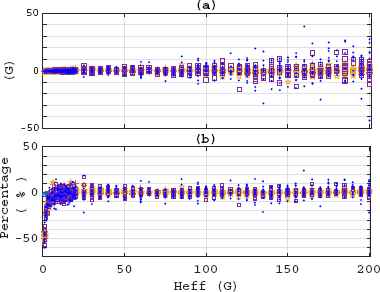
Heff (a) Absolute Error and (b) Percentage Error.
Notice that the same symbols used in Fig. 5 to denote NP levels are used in both Figures 7(a) and 7(b). As expected, the spectra with the highest noise produce the cases with the highest errors. Following the calculated Normal distribution probability for the percentage errors, as shown in Fig. 6, the probability of having a percentage error between 10% and −10% is P(−10% < PE < 10%) = 82.11%, which improves to P(−15% < PE < 15%) = 95.63% and P(−20% < PE < 20%) = 99.29%.
Based on the results shown above, it can be concluded that the use of Machine Learning, specifically Artificial Neural Networks, allows for the determination of the mean longitudinal magnetic field of stars. This can be achieved within an ±20% margin of error 99% of the times for Heff > 1G, even when the Signal to Noise Ratio of the spectra is as low as 11.
The results obtained in this work already represent an important development in the application of ANN on real data. However, our next goal is to expand the database to include variations in all of the parameters that remained fixed in this work, in order to obtain the Heff from real objects. Nevertheless, in this paper, the use of machine learning algorithms has been proven to be a powerful tool in the study of magnetic fields through the analysis of polarized spectra.
Acknowledgments
Part of the results presented here were obtained using the “UNAM Supercómputo - DGTIC” facilities, grant SC16-1-IR-40, the computers from projects CONACyT 153985 and UNAM-PAPIIT 107215 and the computers “Tycho” (Posgrado en Astrofísica, Instituto de Astronomía-UNAM and PNPC-CONACyT).
J.P. Córdova acknowledges the Mexican National Council for Science and Technology (CONACyT) for its financial support, J.C. Ramírez and S.G. Navarro acknowledge financial support from CONACyT grants 240441 and 168078 respectively.
References
Cite this article
TY  - JOUR
AU  - J.P. Córdova Barbosa
AU  - S.G. Navarro Jiménez
AU  - J.C. Ramírez Vélez
PY  - 2018
DA  - 2018/01/22
TI  - Machine Learning for Stellar Magnetic Field Determination
JO  - International Journal of Computational Intelligence Systems
SP  - 608
EP  - 615
VL  - 11
IS  - 1
SN  - 1875-6883
UR  - https://doi.org/10.2991/ijcis.11.1.46
DO  - 10.2991/ijcis.11.1.46
ID  - Barbosa2018
ER  -