
Resolving a portfolio optimization problem with investment timing through using the analytic hierarchy process, support vector regression and a genetic algorithm
- DOI
- 10.2991/ijcis.11.1.77How to use a DOI?
- Keywords
- Stock investment; Portfolio optimization; Analytic hierarchy process; Support vector regression; Genetic algorithm
- Abstract
In the field of financial investment, investing in stocks is relatively easy compared to other investment commodities, since making a profit through buying a stock at a low price and selling it at a higher price is intuitive. However, it is really challenging work for an investor to choose stocks which might be profitable, to determine the capital allocations for these selected stocks or even to time the transactions for stocks. In this study, the analytic hierarchy process (AHP), support vector regression (SVR), and genetic algorithm (GA) are employed to design a three-stage portfolio optimization approach for sequentially solving the portfolio selection, portfolio optimization, and transaction timing. Stocks in the semiconductor and iron and steel subsectors in Taiwan are used to illustrate the procedures for applying the present approach. Based on the investment results from 26 May 2017 to 25 Aug. 2017, the annualized returns on investment are 15.36% and 6.15% for the stock markets of the semiconductor and iron and steel sub-sections, respectively. Both returns are superior to the one-year certificate of deposit of about 1% in Taiwan. Hence, we are confident that the proposed approach can fit the real-world stock market, and thus serve as a valuable, functional tool for an investor.
- Copyright
- © 2018, the Authors. Published by Atlantis Press.
- Open Access
- This is an open access article under the CC BY-NC license (http://creativecommons.org/licences/by-nc/4.0/).
1. Introduction
In the field of financial investment, investing in stocks is relatively easy compared to other investment commodities. However, it is really a challenging work for an investor to choose stocks which might be profitable, as well as determine the capital allocations for these selected stocks. Selecting potentially profitable stocks from the “sea of stocks” in the financial market is a difficult problem.
As shown in Figure 1, an investor will face a difficult problem and dilemma to choose the best investment stock based on three corporations’ financial performance. Therefore, multiple criteria decision-making (MCDM) techniques have been broadly used to evaluate the operating performance of candidate investment corporations, thus selecting investment targets which are expected to be potentially profitable in previous studies.
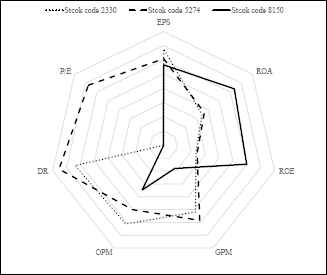
Radar axis labels for the financial performance of corporations.
For example, Wang et al.1 proposed a systematic method to assist organizations in determining the best sustainable development goals partner. They used a super slacks-based model (super SBM) to rank companies, and measured their efficiency, technical, and productivity changes during the past 2012–2015 based on the Malmquist productivity index (MPI) as well as to forecast their future performance in 2016–2019 by using the GM (1,1) model. The optimal green logistics partnerships and their competitiveness levels from 2012 to 2019 were identified through combining the data envelope analysis (DEA) and grey methods.
Hsu2 integrated data envelopment analysis (DEA) and improved grey relational analysis (IGRA) to design a decision-making model, thus measuring the relative efficiencies in order to evaluate the efficiency and operating performance of semiconductor companies listed in Taiwan in 2010. The semiconductor companies are first divided into two groups, i.e. efficient and inefficient. Then, the operating performance of the efficient and inefficient groups are evaluated, respectively, by combining multiple-criterion decision-making (MCDM) VlseKriterijumska Optimizacija I Kompromisno Resenje (VIKOR), IGRA and entropy weight methods. In addition, the author suggests that investors should choose companies with higher efficiency and operating performance as investment targets, rather than only considering the performance rankings of candidate investment targets as in the past.
Song and Guan3 applied a super-efficiency slacks-based measure (SBM) model to assess the e-government performance of environmental protection administrations in 16 cities in Anhui Province, China, according to their three first-level indicators, including the degree of public participation, website service quality, and public satisfaction. Slacks-based measure (SBM) models were applied in their study since the performance of DMUs can be successfully evaluated, and frontier efficiency studies can be more relevant to the business world.
Ghadikolaei et al.4 proposed a hybrid approach to evaluate the financial performance of automotive companies in the Tehran stock exchange (TSE) market. They first utilized the Fuzzy Analytic Hierarchy Process (FAHP) to find the optimal criteria weights. These companies were then ranked through simultaneously applying the Fuzzy VIKOR, Fuzzy Additive Ratio Assessment (ARAS-F) and Fuzzy Complex Proportional Assessment (Fuzzy COPRAS) methods. From the analytical results, they found that the importance of economic value measures was higher than accounting measures in financial performance when evaluating these companies.
Shaverdi et al.5 evaluated the performance of three nongovernmental Iranian banks by constructing an approach that uses multiple criterion decision-making (MCDM) tools, including TOPSIS, VIKOR and ELECTRE, where 21 indexes selected from the BSC concept were evaluated. In addition, they applied the fuzzy analytic hierarchy process (FAHP) to calculate the relative weights of each chosen index, thus tolerating the vagueness and ambiguity of information.
Dong et al.6 and Dong et al.7 utilized multiple preference relations to develop a linguistic multiperson decision-making model (LMDMM). They first relate the fuzzy preference relations and several types of multiplicative preference relations with multigranular linguistic preference relations by using some obtained transformation functions. Then, they apply the fuzzy majority and a 2-tuple ordered weighted averaging operator to design a selection mechanism for the LMDMM. In addition, the conditions for whether their proposed selection approach will satisfy social choice axioms are also discussed. Their proposed approach is quite practical, since there are usually several decision makers who come from different backgrounds and have knowledge in various professional domains. Furthermore, it is easier for decision makers to express their favorites through fuzzy linguistic forms than through exact numerical forms.
The investors must determine the capital allocation for each chosen investment target after picking the investment targets from the “sea of stocks”, i.e. the portfolio optimization problem, with the goal of simultaneously maximizing the overall expected profit, as well as minimizing the overall investment risk. However, the portfolio optimization is an NP-hard problem, since the relationships among these investment targets are complex, as shown in Table 1. In addition, accurately forecasting future stock prices is essential when constructing a portfolio model. Although technical indicators are commonly used to forecast stock prices, their relationship is very complicated, and is difficult to examine, as illustrated in Figure 2.
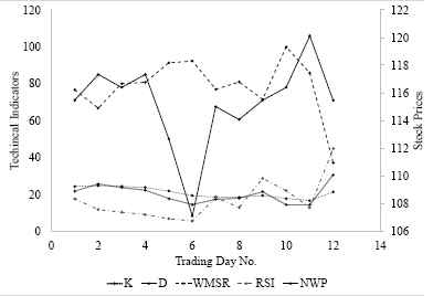
Relationship between stock prices and technical indicators.
| Stock codes | ||||||
|---|---|---|---|---|---|---|
| 2330 | 2408 | 3529 | 3532 | 5269 | ||
| Stock codes | 2330 | 1588.168 | −98.6106 | 4849.608 | 298.1186 | 2421.814 |
| 2408 | −98.6106 | 716.3353 | 369.4055 | 213.7038 | 271.7814 | |
| 3529 | 4849.608 | 369.4055 | 18841.86 | 1038.755 | 9031.88 | |
| 3532 | 283.9073 | 207.8608 | 993.2522 | 319.5198 | 1146.873 | |
| 5269 | 2346.246 | 224.1611 | 8751.73 | 1181.068 | 6316.789 | |
Co-variances of stocks.
Hence, it’s an arduous task to obtain a “hard” optimal solution, i.e. a globally optimal solution, for the portfolio optimization problem with a time constraint, especially when additional constraints are added in the portfolio optimization model. Therefore, soft computing techniques have recently been broadly utilized to acquire a “soft” optimal solution, i.e. a near-optimal solution, in an acceptable time.
For example, Kumar and Mishra8 proposed a method that mixes co-variance principles with an artificial bee colony (ABC) to tackle the portfolio optimization problems algorithm with multiple conflicting objectives so as to speed the convergence with more precision. Several portfolio optimization problems from the OR-library were examined to verify the efficacy and efficiency of their proposed algorithm. Their proposed approach can find various optimal trade-off solutions by simultaneously handling realistic constraints based on the experimental results.
Ni et al.9 improved the traditional particle swarm optimization (PSO) algorithm with dynamic random population topology abstracted into an undirected connected graph that can be randomly generated based on some predefined rules and degrees. The revised PSO can enhance both the communication mechanisms which evolve in the evolutionary process and the solving performance of PSO through tuning the rules and degrees. Several improved PSO algorithms based on the dynamic random population topology were compared to classical PSO variants to solve the generalized portfolio selection model with their experimental data including the weekly indices of the Hang Seng, DAX 100, FTSE 100, S&P 100 and Nikkei 225 during some periods. The implementation results indicated that their proposed dynamic random population topology can indeed notably meliorate the calculation performance of the traditional PSO method.
Metawa et al.10 utilized the genetic algorithm (GA) to propose a self-organizing method to dynamically organize bank lending decisions. Their proposed model simultaneously considers the maximization of bank profit and minimization of the probability of bank default to construct an optimal loan portfolio. In specific, several factors of loan characteristics and creditor ratings are integrated with the encodings of GA chromosomes, thus obtaining the most efficient lending decision.
Seyedhosseini et al.11 hybridized the harmony search (HS) and artificial bee colony (ABC) methods to resolve a portfolio optimization problem formulated by a Markowitz mean-semivariance model. The efficiency and accuracy were evaluated through comparing the efficient frontiers obtained by their proposed method to those yielded by the HS and GA (genetic algorithm) methods. The computational results indicated that their proposed approach is more successful than HS and GA, and can find the optimal solution as well.
Lwin et al.12 extended the Markowitz mean-variance portfolio optimization model by considering the cardinality, quantity, pre-assignment and round lot constraints existing in the real world. They proposed a multi-objective evolutionary algorithm that hybridizes the learning-guided solution generation strategy to promote the efficient convergence by guiding the evolutionary search towards the promising regions of the search space to solve the extended portfolio optimization problem. The public OR-library datasets from seven market indices that involve up to 1318 assets were used to compare their proposed algorithm to four multi-objective evolutionary algorithms, including the non-dominated sorting genetic algorithm (NSGA-II), strength Pareto evolutionary algorithm (SPEA-2), Pareto envelope-based selection algorithm (PESA-II) and Pareto archived evolution strategy (PAES). The results revealed that their proposed approach can significantly outperform the other four multi-objective evolutionary algorithms, providing an efficient frontier of better quality.
Mishra et al.13 applied the multi-objective bacteria foraging optimization (MOBFO) method to resolve the portfolio asset selection (PAS) problem that additionally considers multiple practical constraints, including the minimum buy in threshold, maximum limit and cardinality, in the traditional general PAS. In their study, five benchmark data sets were utilized to compare their proposed method to a set of competitive multi-objective evolutionary algorithms based on the six performance metrics, Pareto front and computational time. Their proposed MOBFO algorithm was able to identify a good Pareto solution while maintaining acceptable diversity, as well as providing adequate solutions for different cardinality constraints.
Hajinezhad et al.14 developed an artificial neural network (NN), called mixed Tabu machine (MTM), where the state transition mechanism is regulated through a Tabu search mechanism in both discrete and continuous search spaces to assist in the searching process, escaping from local minimum states of the energy, and thus finding the global optimum. They utilized the MTM to tackle the portfolio optimization problem, and used the data sets drawn from five capital market indices, including the Hang Seng in Hong Kong, DAX 100 in Germany, FTSE 100 in the UK, S&P100 in the USA and Nikkei 225 in Japan, to verify the efficiency of the MTM. The experimental results revealed that their proposed MTM can intelligibly yield excellent results within a very small CPU time.
From the above literature review, we can find that the multiple-criterion decision-making (MCDM) techniques are common tools for assessing and ranking the operating performance of corporations, and thus picking the so-called “good” firms with high performance. In addition, the AHP method is infrequently used compared to the DEA, TOPSIS, and VIKOR etc. Next, soft computing techniques, e.g. the genetic algorithm (GA), particle swarm optimization (PSO), artificial bee colony (ABC), harmony search (HS), and bacteria foraging optimization approaches, as well as their variants, are broadly used to obtain near-optimal solutions for the portfolio optimization problem. However, the probability, i.e. risk, of the investors being unable to acquire the estimated profit, is not considered. Moreover, the “portfolio selection”, “portfolio optimization”, and even “stock transaction” are treated as three independent problems, although these problems rely on each other. Therefore, in the present study, the analytic hierarchy process (AHP), support vector regression (SVR) and a genetic algorithm (GA) are applied to develop a three-stage portfolio optimization approach to tackle the above three problems simultaneously.
As to the advantages of the proposed approach, the AHP can help an investor easily select investment stocks while simultaneously considering multiple financial indexes and arbitrarily altering their relative importance according to an individual’s preferences based on financial reports. Next, the SVR tool can assist a user in exploring the complex mentalities of investors in the stock market, thus more precisely predicting future stock prices by investigating the complicated inherent hidden relationship between technical indicators and stock prices. Finally, an investment portfolio model that takes both investment profit and risk into consideration is given, and the optimal portfolio is provided for an investor by efficiently resolving the complicated nonlinear mathematical model via the GA. Furthermore, the best transaction timing regarding each stock can be definitely determined for the investor.
The remainder of the paper is organized as follows. First, the methods utilized in this study are briefly introduced. The three-stage approach is then proposed in the next section. Later, a case study on investing in the semi-conductor and steel sections in the Taiwan stock market is presented to demonstrate and validate the proposed method. Finally, the conclusions and future research recommendations are given.
2. Research Methodology
In this study, the AHP, SVR, and GA are used to develop our integrated procedure. The important reasons for applying these methods are explained as follows.
Firstly, the AHP, instead of the DEA, TOPSIS or VIKOR, is used to tackle the MCDM problems, since the original financial indexes can be fed into the AHP with simple mutual comparisons. The complex scoring process of experts or recognizing the best and worst cases are not needed. The user can arbitrarily set the importance of each criterion (financial index) based on his/her preference. In addition, the AHP is quite suitable in a personal, but not a group’s, decision-making situation, and it is quite suitable for our research objective, which is to develop a stock investment procedure for an individual investor, rather than for investment institutions.
Secondly, the main advantage of the support vector machine (SVM) is that it can overcome a problem whose observations relate to a lot of input variables, i.e. a problem with high dimensionality15. In addition, SVR has several advantages of the SVM, while fitting the data with a continuous-valued function16. Therefore, the SVR is thought to be very favorable for constructing a forecasting model for stock prices based on a group of technical indicators.
Finally, the GA has three main advantages: (1) mathematical requirements for the optimization problems are minimized/avoided; (2) the GA can perform a global search in probability with very great effectiveness due to the evolution operators’ ergodicity; (3) the hybridizing of GA with domain-dependent heuristics is highly flexible17. Consequently, the GA is employed to optimize the portfolio, which is a very complicated non-linear NP-hard problem.
The above three methods are briefly introduced in this section.
2.1. Analytic hierarchy process
The analytic hierarchy process (AHP), introduced by Satty18 is an effective structural tool for organizing and analyzing complex decision-making problems. In the AHP, a decision-making problem must be decomposed into a hierarchy of sub-problems (criteria) where each sub-problem can be analyzed independently and is more easily comprehended than the original problem. Suppose a decision-making problem has m decomposed criteria and a decision maker has n alternatives, as shown in Figure 3. There are three steps in the AHP as follows.
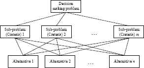
An example of AHP.
Step 1: Calculating the criteria vector
The AHP creates a criterion comparison matrix A (m × m) by comparing the relative importance of the criteria. The element aij in A represents the importance of the ith criterion relative to the jth criterion. The ith criterion is more important than the jth criterion if aij > 0, and aij < 0 represents the opposite situation. If two criteria have the same importance, then the element aij equals one. The normalized criterion comparison matrix Anorm (m × m) is then calculated based on the following formula:
Finally, the criterion vector w (m-dimensional column vector) can be obtained based on the following equation:
Step 2: Computing the score matrix
First, each alternative k is compared to the alternative l with respect to the ith criterion to form the element
Next, the score matrix S (n × m) can be acquired as follows:
Step 3: Alternative ranking
The global score vector v (n × 1) is calculated by
2.2. Support vector regression
In the real world, research frequently has to model the functional relationship between some inputs and one or more output variables. The function modeling task becomes more complex and difficult when the inputs have non-linear effects on the output. In order to resolve the problem of non-linear regressions Vapnik et al.19 and Drucker et al.20 introduced a technique for the regression, called support vector regression (SVR). Suppose we want to construct a regression model to describe the relationship between Q pairs of the inputs Xk = (xk1, xk2, ..., xkn) ∈ Rn is a vector in n dimensions, and its corresponding output yk ∈ R. The original inputs Xk (k = 1, 2, ..., Q) are first transformed into the ϕi (Xk) in a higher-dimensional space (m dimensions). Then, we intend to approximate the weight for the transformed inputs ϕi (Xk) to construct the linear regression model for acquiring the predicted output y′k as follows:
In other words, the loss can be re-stated as follows:
Notably, the error of the real value yk being above and below the predicted y′k is evaluated by the non-negative slack variables, ξi and ξ′i, respectively. Then, Vapnik22,23 defined the empirical risk minimization problem as follows:
Next, the optimality can be obtained by taking the partial derivative of LP with respect to the primal variables to its saddle point as follows:
Define K(Xk, Xl) ≡ Φ(Xk) · Φ(Xl) be the kernel function, then Equation (14) is replaced by Equations (15), (17), and (18) to yield the simplified dual form LD as follows:
Maximize
Notably, some kernel functions which are commonly used include the linear, polynomial (homogeneous), polynomial (inhomogeneous), radial basis function, hyperbolic tangent, etc. Furthermore, the “support” vector is the data (Xk, yk) whose corresponding λi or λ′i is not zero. Finally, the optimal approximation Ŵ for the weight vector W can be derived by optimizing the Lagrangian as follows:
Notably, the index k only carries out for the support vectors whose total number is ns. As for the optimal approximated bias ŵ0, the Karush–Kuhn–Tucker (KKT) conditions24,25 are applied to get the approximation of w0 as follows:
Notably, the support vectors which are unbounded and make the Lagrangian multipliers fulfill 0 < λk < C and
2.3. Genetic algorithm
Based on the mechanism of evolution, Holland29 developed a broadly used heuristic for acquiring near-optimal solutions for an optimization problem, called the genetic algorithm (GA). To apply the GA, the first step is to represent the solution for a problem through using an individual, called a chromosome, which uses the coding scheme. Then, we must define an objective function to evaluate the fitness of a chromosome for the optimization problem. Next, the selection mechanism is designed to choose the so-called better chromosomes to make up the crossover pool, called parents. In addition, the crossover mechanism is devised to create offspring chromosomes, called children, by matching the parents and exchanging gene information between the parents. To simulate genetic mutations in nature, a mutation procedure is also developed. The principal and execution procedure for a general GA can be stated as follows:
- Step 1:
Design the genetic representation method for producing the chromosomes for an optimization problem.
- Step 2:
Define the fitness function based on the objective function.
- Step 3:
Generate a population of chromosomes, usually randomly or according to a certain method that is especially designed based on some principles in advance.
- Step 4:
Obtain the solution by de-coding each chromosome in the population to thus yield the corresponding fitness value for each chromosome.
- Step 5:
Select some chromosomes to form the crossover pool by applying a certain rule, e.g. Russian wheelset, based on the fitness value of each chromosome in the population.
- Step 6:
Randomly pair two chromosomes in the crossover pool to create some paired parents.
- Step 7:
Apply the crossover mechanism to each pair of parents in the crossover pool to produce their offspring chromosomes.
- Step 8:
Utilize the mutation mechanism on these offspring chromosomes.
- Step 9:
Evaluate the fitness values for these offspring chromosomes and randomly select the survival chromosomes from the original chromosomes, i.e. the chromosomes in the population as stated in Step 4, and the offspring chromosomes based on their fitness, thus forming the new population, i.e. the population in Step 4 has been updated.
- Step 10:
Stop and yield the final optimal solution (chromosome), i.e. the chromosome with the best fitness, if the termination criteria are satisfied; otherwise, go to Step 4.
3. Proposed Three-Stage Portfolio Optimization Procedure
This study develops a portfolio optimization procedure. The steps are graphically summarized in Figure 4, and are explained in detail in the following sub-sections.
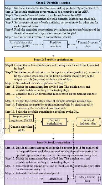
Proposed procedure.
3.1. Portfolio selection
In the first stage, the analytic hierarchy process (AHP) is used to rank the candidate corporations based on their financial reports. Notably, the “decision-making problem” (goal) in Figure 3 is to “select stocks” which are thought of as profitable, and the “sub-problems” corresponding to the “decision-making problem” illustrated in Figure 3 are the financial indexes considered in a study. Next, the relative importance of financial index A (sub-problem A) to financial index B is set IMA / IMB, where IMA and IMB are the importance of financial index A and financial index B, respectively, according to the preferences of the individual investor. The relative performance of corporation A to corporation B for financial index C is set as
The candidate corporations considered in the AHP then can be ranked by synthesizing the performance of the financial indexes of corporations respect to the goal (decision-making problem), i.e. to select stocks. Notably, corporations that have any negative financial index where the index is of the “larger the better” type, e.g. a negative EPS, must be excluded from further analysis by the AHP and the succeeding stages.
3.2. Portfolio optimization
First, the technical indicators and trading data are gathered for the stocks issued by the corporations selected by the AHP in Stage 1. For each selected stock and each trading day, the data are then arranged by making the technical indicators the input variables (predictors) as well as letting the closing stock price of the trading day that is behind the current trading day with a decision-making period, e.g. five trading days, be the output variable (response) to form a row of data.
The data in each column are then normalized, and the arranged normalized data are divided into two parts according to their trading days. The arranged normalized data during the investment period form the validation (the second part) data, and the remaining arranged normalized data make up the first part. In addition, the first part data are further randomly divided into the training and test data based on a proportion.
The support vector regression (SVR) tool is then utilized to construct the forecasting model by using the training and test data, and the cross validation technique is applied to evaluate the forecasting performance. By tuning the parameters in the SVR, the optimal SVR model can be established.
Based on the technical indicators of current decision-making (trading) day i for the stock j selected in the portfolio in the first stage during the investment period, the well-structured SVR model is applied to the validation data to predict the closing stock price of the next decision-making day with a decision-making period. Define the risk that the expected profit cannot be attained as
The genetic algorithm (GA) approach is then implemented for the portfolio optimization problem as formulated in Equations (28) and (29), thus obtaining the optimal capital allocations for the stocks selected in the portfolio for each decision-making day (i = 1,2,…,v) in Equation (29).
3.3. Stock transaction
Through comparing the optimal capital allocations on decision-making day i to the optimal capital allocations obtained on the previous decision-making day i-1, the investor can decide the share amount that should be bought or sold for each stock j in the portfolio on each decision-making day i as shown as follows:
The buying or selling of stocks is implemented on the next trading day after the decision-making day. Finally, the transaction profit associated with each decision-making day can be obtained, thus yielding the final investment profit during the investment period.
4. Case Study
4.1. Constructing the portfolio
In this study, the stocks in semiconductor and iron and steel sub-sections of the Taiwan stock market are considered. The period of study is from 1 Jan. 2012 to 13 Jun. 2017. First, the financial reports announced at the end of the first quarter in 2017 were gathered from the TEJ (Taiwan Economic Journal)* database for all the (222) corporations which issue stocks in the semiconductor sub-section in Taiwan.
Among the financial indexes, seven important indicators, including the earnings per share (EPS), return on assets (ROA), return on equity (ROE), gross profit margin (GPM), operating profit margin (OPM), debt ratio (DR), and price-earnings ratio (P/E) are chosen as the criteria in AHP. The selection of profitable stocks in a portfolio through the AHP then can be described as a decision-making problem consisting of seven sub-problems as shown in Figure 5.
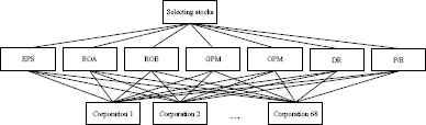
The description of the decision-making problem in the AHP for selecting stocks.
Notably, the total number of the candidate corporations which are further analyzed is 68, after eliminating the corporations which have a negative, “the larger the better” financial index. Each criterion (financial index) is considered as important as the other criterion (financial index). Hence, all of the elements aij s that represent the importance of the ith criterion relative to the jth criterion are set as 1, thus comprising the 7 × 7 comparison matrix A. Therefore, the normalized criteria comparison matrix Anorm then can be calculated according to Equation (1), and the criteria vector w (seven-dimensional column vector) is obtained based on Formula (2). Next, each alternative (corporation) k is compared to the alternative (corporation) l with respect to the ith criterion (financial index) by the element
Ten corporations are considered in this study, and the execution result of the Expert Choice 11† is shown in Figure 6. The ten stocks include the stocks of codes 3529, 6510, 6462, 2408, 5274, 8150, 5269, 2330, 6568, and 3532 according to their priorities to the global goal, are selected.
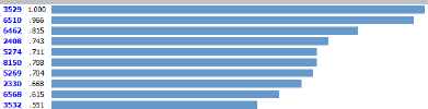
The selected ten stocks based on the execution result of the Expert Choice 11 for the semiconductor sub-section in Taiwan’s stock market.
4.2. Optimizing the portfolio
The technical indicators and trading data of the selected ten stocks as shown in Figure 5 were first collected from the C-Money‡ and TEJ§ databases during 1 Jan. 2012 to 25 May 2017. Notably, there are 16 technical indicators, (1) the 10-day moving average, (2) 20-day bias, (3) moving average convergence/divergence, (4) 9-day stochastic indicator K, (5) 9-day stochastic indicator D, (6) 9-day Williams overbought/oversold index, (7) 10-day rate of change, (8) 5-day relative strength index, (9) 24-day commodity channel index, (10) 26-day volume ratio, (11) 13-day psychological line, (12) 14-day plus directional indicator, (13) 14-day minus directional indicator, (14) 26-day buying/selling momentum indicator, (15) 26-day buying/selling willingness indicator, and (16) 10-day momentum, considered in this study in accordance with Kim and Han30, Kim and Lee31, Tsang et al.32, Chang and Liu33, Ince and Trafalis34, Huang and Tsai35, Lai et al.36, and Hsu37.
For each trading day, the sixteen technical indicators along with the closing stock price of the trading day that is apart from the current trading day with a decision-making period are arranged into a row. These technical indicators and closing stock price serve as the input variables and output variable, respectively.
The data in each column are then normalized into a range between 0 and 1 according to the maximum and minimum values of the corresponding column. Next, the arranged normalized data during 1 Jan. 2012 to 25 May 2017, i.e. the model building period, contain 8641 data points to form the part (I) dataset. In addition, the part (II) dataset, consisting of the arranged normalized data during 26 May 2017 to 25 Aug. 2017, i.e. the investment period, forms the validation data. The training and test data are generated by randomly dividing the part (II) data based on a proportion of 3:1. Therefore, the training, test, and validation data contain 6481, 2160, and 650 data points, respectively.
The LIBSVM ** SVR tool is then applied to the training and test data to construct the forecasting model where the forecasting performance is evaluated through the cross-validation technique, and the parameters in the SVR are optimized by the grid-search approach25. The important parameters C, Gamma, and Epsilon in SVR are then optimally set at 32, 0.707106781187, and 0.00390625 respectively. In addition, the radial basis function (RBF) kernel is used. The obtained SVR model provides R2 and MSE of 0.994363 and 0.00005428 for the training data, and 0.991832 and 0.00006052 for the test data. These values reflect the fact that the SVR can model the non-linear functional relationships between the inputs (technical indicators) and outputs (stock closing prices) with sufficient accuracy and can be used in forecasting the stock prices in the future.
Forecasting the closing stock price of the next decision-making (trading) day with a decision-making period, based on the technical indicators of the current decision-making (trading) day during the investment period, 26 May 2017 to 25 Aug. 2017, via the well-constructed SVR model, the Evolver 7†† software of GA is implemented to resolve the portfolio optimization problem as shown in Equations (28) and (29) to determine the optimal capital allocation for each stock in the portfolio on the next decision-making day during the investment period.
The target profit TP and the very larger number M in Equation (27) are set as 0.02048% and 1,000,000, respectively. Notably, the one-year certificate of deposit of the Taiwan bank is 1.065%, and the target profit is set at 1.065%/52=0.02048% since the capital allocations in the portfolio are optimized weekly. The population size, crossover rate, and mutation rate in GA are set at 50, 0.5, and 0.15, respectively. The GA procedure is implemented 10 times for each decision-making day, and Table 2 illustrates the optimal capital allocations for the stocks in the portfolio on some decision-making days.
| Decision making day | Stock code | Capital allocations |
|---|---|---|
| 2017.05.26 | 2330 | 0 |
| 2408 | 0 | |
| 3529 | 0.004100 | |
| 3532 | 0 | |
| 5269 | 0 | |
| 5274 | 0 | |
| 6462 | 0.114866 | |
| 6510 | 0 | |
| 6568 | 0.881033 | |
| 8150 | 0 | |
|
|
||
| 2017.06.02 | 2330 | 0 |
| 2408 | 0 | |
| 3529 | 0.010048 | |
| 3532 | 0.989952 | |
| 5269 | 0 | |
| 5274 | 0 | |
| 6462 | 0 | |
| 6510 | 0 | |
| 6568 | 0 | |
| 8150 | 0 | |
|
|
||
| 2017.06.09 | 2330 | 0 |
| 2408 | 0.024577 | |
| 3529 | 0 | |
| 3532 | 0.893456 | |
| 5269 | 0 | |
| 5274 | 0.081967 | |
| 6462 | 0 | |
| 6510 | 0 | |
| 6568 | 0 | |
| 8150 | 0 | |
The optimal capital allocations for the stocks in the portfolio on some decision-making days.
4.3. Transacting stocks
During the investment period, the optimal capital allocations on each decision-making day are compared to the optimal capital allocations obtained the previous decision-making day, thus calculating the amount of stock in the portfolio to be bought or sold based on Equation (30). In addition, the total investment capital CAP is set at one million new Taiwan dollars.
Take the decision-making day 9 Jun. 2017 as an example, the share amount for the stock coded 3532 which should be bought or sold is calculated as
By applying a similar procedure to each stock in the portfolio for each decision-making day, the final investment profit then can be obtained.
4.4. Evaluating performance
There are 64 iron and steel corporations which issue stocks on the Taiwan stock market. The final return of investment during the same investment. Similarly, the investment procedures illustrated in Sections 4.1 to 4.3 are also applied to the stocks issued in the iron and steel sub-section of the Taiwan stock market. The parameters C, Gamma, and Epsilon in SVR are set at 8, 1, and 0.00390625, which are obtained by the grid-search approach25, and the RBF kernel is adopted. The GA parameters, including the population size, crossover rate, and mutation rate are set at 50, 0.5, and 0.15, respectively. Table 3 summarizes the investment performance of the stocks of the semiconductor and iron and steel sub-sections in Taiwan’s stock market.
| Stock sub-section | Semiconductor | Iron & steel |
|---|---|---|
| Investment period | 2017.05.26~2017.08.25 | 2017.05.26~2017.08.25 |
| Initial capital | 1,000,000 | 1,000,000 |
| Final capital | 1,038,395 | 1,015,446 |
| Three-month ROI | 3.8395% | 1.5446% |
| Annualized ROI | 15.36% | 6.18% |
Summary of investment performance.
According to Table 2, the annualized returns of investment are 15.36% and 6.15% for the semiconductor, and iron and steel sub-sections, respectively. The interest rate for the one-year certificate of deposit in Taiwan is about 1%. Hence, the implementation results confirm that the proposed approach is a practical investment tool in the stock markets of the real world.
5. Conclusions
Portfolio optimization problems have been broadly investigated in previous studies. However, the optimization models usually only considered whether an investor can obtain his/her estimated profit. But the issue regarding the investment risk, i.e. the possibility that an investor cannot get his/her desired estimated profit, which is more important to the investor, is not considered. Next, most studies have independently treated the “portfolio selection”, “portfolio optimization”, and “stock transaction”. However, the above three problems influence each other in fact. Therefore, this study utilizes the analytic hierarchy process (AHP), support vector regression (SVR) and genetic algorithm (GA) to design a three-stage portfolio optimization procedure in order to systematically resolve these simultaneously.
The proposed approach is demonstrated by a case study of investing in the stocks of the semiconductor and iron and steel sub-sections in the Taiwan stock market. Based on the experimental results, the annualized returns of investment can reach 15.36% and 6.15% for the semiconductor and iron and steel subsections, respectively, which are much better than the one-year certificate of deposit (about 1%) in Taiwan,. Therefore, our proposed approach can be considered a practical and useful tool for investing in stocks in the real-world stock market.
In summary, the proposed approach has the following contributions: 1. an investor can take account of several financial indexes simultaneously, and arbitrarily changing their relative importance based on his/her own preferences; 2. the performance of stock prices in the future can be forecast by implicitly investigating the mentality of public investors by using explicit technical indicators; 3. an individual can take into account both investment profit and risk, thus establishing his/her optimal investment portfolio; 4. the optimal timing of transacting stocks can be clearly settled.
The possible future research can have several directions, e.g. (1) studying the relationship between the performance of stocks and corporations’ operational efficiency, (2) the practical considerations of stock transactions such as the segmentation of stock shares and transaction costs, and (3) optimizing the settings of parameters in the SVR and GA.
Acknowledgements
The author thanks the Minghsin University of Science and Technology, Taiwan, R.O.C., for supporting this study under Contract No. MUST-107BA-1.
Footnotes
References
Cite this article
TY  - JOUR
AU  - Chih-Ming Hsu*
PY  - 2018
DA  - 2018/05/28
TI  - Resolving a portfolio optimization problem with investment timing through using the analytic hierarchy process, support vector regression and a genetic algorithm
JO  - International Journal of Computational Intelligence Systems
SP  - 1016
EP  - 1029
VL  - 11
IS  - 1
SN  - 1875-6883
UR  - https://doi.org/10.2991/ijcis.11.1.77
DO  - 10.2991/ijcis.11.1.77
ID  - Hsu*2018
ER  -