
Group Decision Making with Incomplete Reciprocal Preference Relations Based on Multiplicative Consistency*
Etienne E. Kerre, Fuzziness and Uncertainty Modeling Research Unit B-9000 Gent, Belgium.
- DOI
- 10.2991/ijcis.11.1.78How to use a DOI?
- Keywords
- Fuzzy set; Group decision making; Reciprocal preference relation; Incomplete preference relation; Multiplicative consistency
- Abstract
This paper comprises a new iterative method for multi-person decision making based on multiplicative consistency with incomplete reciprocal preference relations (IRPRs). Additionally, multiplicative transitivity property of reciprocal preference relation (RPR) is used at the first level to estimate the unknown preference values and get the complete preference relation, then it is confirmed to be multiplicative consistent by using transitive closure formula. Following this, expert’s weights are evaluated by merging consistency and trust weights. The consistency weights against the experts are evaluated through multiplicative consistency investigation of the preferences given by each expert, while trust weights play the role to measure the level of trust for an expert. The consensus process determines whether the selection procedure should start or not. If it results in negative, the feedback mechanism is used to enhance the consensus degree. At the end, a numerical example is given to demonstrate the efficiency and practicality of the proposed method.
- Copyright
- © 2018, the Authors. Published by Atlantis Press.
- Open Access
- This is an open access article under the CC BY-NC license (http://creativecommons.org/licences/by-nc/4.0/).
1. Introduction
Decision making (DM) is an intellectual procedure which is used to select the best option(s) amongst several different options, it initiates when we have to do something but do not know what. Every individual faces DM situations in his/her daily life: common examples for these situations are shopping, to choose what to eat, and deciding whom or what to vote for in an election or referendum, and can be categorized in several different groups according to certain characteristics as the source(s) for the information and the preference representation formats that are used to solve the decision problem. In our framework, the selection of the best alternative(s) from a predetermined set X = {x1, x2, x3, …, xn}, n ⩾ 2 of possible alternatives is the goal.
DM is not only the case for a single expert, where he/she compares a finite set of alternatives and construct a preference relation, but some decision problems have to be solved by a group of experts who work together to find the best alternative(s) from a set of feasible alternatives. This decision making with multiple experts is called group decision making (GDM) or also known as multi-person decision making. To solve a GDM problem appropriately, two key processes play an essential role:
- (i)
consensus process;
- (ii)
selection process.
The prior is an iterative process which is composed of several consensus rounds, where the experts accept to negotiate diverse sentiments to have an acceptable level, but a unanimous or full consensus is often not achievable in practice13. After getting the experts’ opinions close enough, the selection process takes place which aims to rank and select (a) suitable alternative(s) from a given set of feasible alternatives. When a number of experts interact to reach a decision, each expert may have exclusive inspirations or objectives and a different decision procedure, but has a common interest in approaching to select the best option(s).
In modern era, various consensus models have been proposed in literature for GDM against a number of preference relations2,9,12,25. However, there may arise some situations for DM problems in which experts are unable to provide precise and complete assessments due to the pressure to make a quick decision, Complexity, or incomprehensive information against the problem to be explained, such situations result in incomplete fuzzy preference relations (IFPRs) i.e., some preference values are missing. GDM in IFPRs environment has been receiving an intensive interest of researchers, and various procedures have been presented to determine unknown preference values17. Such as, a least squared procedure was proposed by Gong8 in 2008 to determine the priority vector for GDM in incomplete preference relations’ (IPRs) environment. In 2010, a goal programming model was presented by Fan and Zhang7 for GDM to deal with IPRs in three formats. In 2013, Xu et al. proposed logarithmic least squares method to evaluate the priority weights in GDM dealing with IFPRs and develop the acceptable fuzzy consistency ratio20. Xu and Wang21 in 2013, presented eigenvector method to repair an IFPR with consistency test relation. In 2015, Xu et al.22 presented a least deviation method to evaluate the priority weights for GDM in IRPRs environment. In 2015, the trust based consensus model and aggregation method for GDM were investigated by Wu et al.19 in the context of incomplete linguistic information.
Moreover, consistency is an important issue to accept when data are provided by the experts5,10 and is linked to the transitivity property. In 2007, Herrera-Viedma et al.12 presented an additive consistency based iterative scheme to evaluate the missing preferences in IFPRs. In 2008, Alonso et al.1 extended the idea proposed by Herrera-Viedma et al.12 to investigate the missing information against several preference formats. In 2014, a consensus based model was proposed by Wu and Chiclana18 for multiplicative consistency of reciprocal intuitionistic preference relations and discussed its application to estimate the unknown preference degrees. In 2015, a confidence consistency driven approach was proposed by Ureña et al.16 to handle GDM problems with incomplete reciprocal intuitionistic preference relations. This approach deals with confidence level and implemented for both consistency and confidence in the determination procedure. In 2015, Ashraf et al.3 proposed a new method for GDM with IFPRs based on T-consistency and the order consistency, where T stands for a triangular norm. In 2017, Xu et al.23 developed a consensus based model for hesitant FPRs and used it in water allocation management as an application.
To achieve an acceptable consensus level, feedback mechanism plays an important role in certain consensus measures6,25,26,27. In 25, Zhang et al. developed a consensus building method based on multiplicative consistency for GDM with IRPRs. Inspired by the work of Zhang et al.25, we observed that the multiplicative transitivity property i.e.,
In this paper, we present an improved method for consensus building in group decision making based on multiplicative consistency with IRPRs. At the first step, we evaluate the missing preferences of IRPRs based on the multiplicative transitivity. Then, we construct the modified consistency matrices of experts which satisfy the multiplicative consistency and measure the level of consistency. The degrees of importance are assigned to experts based on consistency weights aggregated with trust weights. The proposed method provides us with a valuable way for consensus building in group decision making based on multiplicative consistency with incomplete preference relations.
The rest of the paper is organized as follows. In Section 2, we focus on some preliminaries used in this paper. In Section 3, we present a new procedure to estimate the missing preferences in incomplete preference relations based on the multiplicative transitivity and construct the modified consistency matrices which satisfy the multiplicative consistency. In Section 4, the proposed GDM process is detailed. In Section 5, an example is given to illustrate the realism and achievability of the proposed technique. Last section includes some conclusions.
2. Preliminaries
In 1965, Zadeh introduced fuzzy set theory 24, designated with a number between 0 and 1, to cope with imprecise and uncertain information working in complex situation.
Definition 1. Fuzzy Set24:
A fuzzy set A on the universe of discourse X is a mapping from X to [0,1]. and is denoted by A = {(x, A(x))}. For any x ∈ X, the value A(x) is called the degree of membership of x in A i.e., A(x) =Degree(x ∈ A), and the map A: X → [0, 1] is called a membership function.
Definition 2. Reciprocal Preference Relation (RPR)5:
An RPR R on a set X of alternatives X = {x1,x2, ..., xn} is characterized by a membership function R(xi, xj) = rij, satisfying rij + rji = 1 for all i, j ∈ {1,2,3, .., n}.
An RPR may be conveniently denoted by matrix R = (rij)n×n, with the following interpretations:
Definition 3. Incomplete Reciprocal Preference Relation (IRPR)11:
An IRPR R = (rij)n×n carries at least one unknown preference value rij for which the expert does not have a clear idea of the degree of preference of alternative xi over the alternative xj.
Definition 4. Multiplicative Transitivity Property15:
An RPR R = (rij)n×n on a finite set X of alternatives is said to be multiplicative transitive if and only if
3. Evaluating missing preferences
This section puts forward a new scheme to estimate the unknown preference values in an IRPR based on multiplicative transitivity. Moreover, the proposed procedure is used to construct a multiplicative consistent matrix.
So as to determine missing preferences in an IRPR R = (rij)n×n, the pairs of alternatives for known and unknown preferences are signified in form of following sets:
New sets of the pairs of alternatives for known and unknown preference values are evaluated as follows:
After having a complete RPR, it needs to be fully multiplicative consistent RPR
4. Iterative procedure for GDM
Now we turn towards our major task to develop a GDM procedure in IRPRs environment. In this section, a new step-by-step algorithm is presented for GDM based on multiplicative consistency. An explanatory example is given to validate the technique. For ease, the structure of the resolution process is also shown in Figure 1.
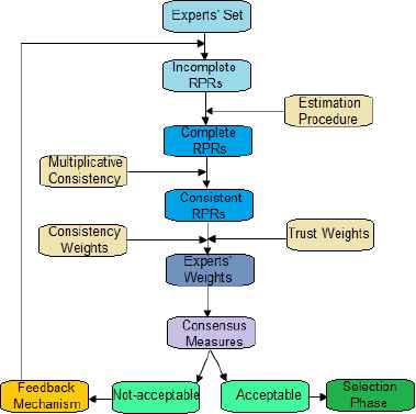
Resolution process for GDM with IFPRs
Suppose that there are n alternatives x1,x2,...,xn and m experts E1,E2,...,Em. Let Rq be the fuzzy preference relation for the expert Eq shown as follows:
4.1. Estimating missing preferences
To determine the missing preference values of an IRPR Rq given by the expert Eq, initially, the sets Kq and Uq of pairs of alternatives for known and unknown preferences are introduced as in (4) and (5) respectively. After this, the multiplicative transitivity based preference values are estimated by using (7)–(11) to construct the complete RPR Rq.
4.2. Consistency measures
After evaluating the complete RPRs, their parallel multiplicative consistent RPRs
- 1.
Multiplicative consistency index (MCI) of a pair of alternatives is determined by using:
where - 2.
MCI associated to a particular alternative xi, 1 ⩽ i ⩽ n, of an RPR is evaluated by:
with MCI(xi) ∈ [0,1]. When MCI(xi) = 1 all the preferences involving the alternative xi are fully consistent, otherwise, the lower MCI(xi) the more inconsistent these preference values are. - 3.
Finally we determine MCI of an RPR Rq by taking the average of all MCI of alternatives xi:
with MCI(Rq) ∈ [0,1]. When MCI(Rq) = 1 the preference relation Rq is fully consistent, otherwise, the lower MCI(Rq) the more inconsistent Rq is.
As soon as the MCI is computed in three levels using expressions (13)–(15), it is rational to assign the higher weights to the experts against the preference relations with larger consistency degrees respectively. Hence, consistency weights can be assigned to the experts by using the relation:
4.3. Allocating weights to experts
The trust weight tw(Eq) is the degree of trust on each expert by others such that
4.4. Consensus measures
After having the RPRs with complete information, it is necessary to measure the consensus among the experts. Regarding this, similarity matrices
- 1.
At first level, the consensus degree on a pair of alternative (xi,xj), denoted by codij is defined to estimate the degree of consensus amongst all experts on that pair of alternatives:
- 2.
At second level, the consensus degree on alternative xi, denoted by CoDi is defined to determine the consensus degree amongst all the experts on that alternative:
- 3.
At third level, the consensus degree on the relation, denoted by CoR is defined to calculate the global degree of consensus amongst all the experts judgments:
Once the global consensus level among all the experts is reached, it requires to compare with a threshold consensus degree η, generally settled in advance depending upon the nature of problem. If CoR ⩾ η, this shows that an acceptable level of consensus has been obtained, and the decision process begins. Otherwise, the consensus degree is not stable, and feedback mechanism is originated.
4.5. Feedback mechanism
The central aim of feedback mechanism is to provide comprehensive knowledge to experts, so as to change their opinions acceptably to enhance the consensus degree. When consensus is not sufficiently high, then we have to identify the preference values that are to be changed, and following formula helps us in this regard:
4.6. Accumulation phase
It may quite frequently happen that the preference degree set forth by each expert is weighted differently. As soon as the weights for the experts are estimated, their preferences need to be accumulated into a global one. Determine the collective matrix RC against all experts, shown as follows:
4.7. Selection phase
After reaching a satisfactory consensus degree amongst all experts, the selection process is initiated to rank all the alternatives in order to select the best option. For a consistent RPR
5. Numerical example
This section deals with a numerical example taken from 25 in order to demonstrate the process of the proposed method and its effectiveness.
Consider that four experts E1,E2,E3 and E4 from different fields are requested to select the best alternative out of four alternatives x1,x2,x3,x4. The four experts give their RPRs as follows:
The threshold consensus level η settled in advance is 0.80. Now, we perform the following steps to evaluate the result:
Step-i: Estimating the missing preferences
Initially, all the missing preference values need to be determined using the multiplicative transitivity property mentioned in Section 1.
Taking R1, for example. The sets of pairs of alternatives for known and unknown preference values are determined as follows:
All the missing preference values are calculated under the use of (7)–(11) to complete the given IRPR. Hence, the complete RPR R1 against expert E1 is obtained as follows:
Similarly, the complete form of R2 can be obtained and given as:
Step-ii: Consistency analysis
Consistency analysis is being conducted to allocate consistency weights to the experts. For this purpose, all complete RPRs are to be converted into their multiplicative consistent forms by using (12), and are given below:
The significant MCI values of the experts are evaluated using (13)–(15), as:
Finally, the consistency weights to the experts are computed by using (16), as:
Step-iii: Weights to experts
Primarily, all experts are assigned the same trust weights: tw(E1) = 1, tw(E2) = 1, tw(E3) = 1 and tw(E4) = 1. Therefore, the weights of the experts remain the same in the first round as the consistency weights based on (17), as:
Step-iv: Consensus measures
After getting complete RPRs, a mutual similarity relation is computed by aggregating the different similarity matrices among the experts using (18)–(19). Then, the consensus measures are computed at the three levels using (20)–(22).
- 1.
On pair of alternatives:
- 2.
On alternatives:
- 3.
On relation:
Now, the threshold consensus degree η settled in advance is compared with global consensus degree CoR of the relation; CoR > η. This indicates that the given consensus degree is acceptable amongst the experts, and we have to enter into accumulation phase.
Step-v: Accumulation phase
Step-vi: Selection phase
The relation RC obtained in (26) is clearly multiplicative consistent, therefore, apply (25) to estimate the ranking value Rv(xi) of alternative xi, 1 ⩽ i ⩽ 4 as follows:
To validate the effectiveness of our proposed method, we compare the results with Zhang et al.25 model which yielded the same results i.e., x2 > x1 > x3 > x4 as ours. But the aggregated matrix obtained by our method is multiplicative consistent at least correct to three decimal places which can further be extended i.e., if we take i = 1 and k = 2, the preference value in aggregated matrix RC is r12 = 0.4992 and the multiplicative consistency requires the same or closed output to r12 by
6. Conclusion
In this paper, an improved hybrid consensus method for GDM problems based on incomplete RPRs is proposed. The multiplicative transitive property is used to estimate the missing values and transitive closure formula is used to make the matrices multiplicative consistent. The weights of the experts are obtained from the consistency analysis and a calculation of degree of trust. Rationally, the experts with high level of consistency and substantial trust degree should have to assign large weights, in order carry more importance in the aggregation process. Additionally, a feedback mechanism making advice to experts subject to their trust weights and consistency weights was proposed which can accelerate the execution of a higher consensus degree. After reaching a satisfactory consensus degree amongst all experts, the selection process is initiated to rank all the alternatives in order to select the best option. Some numerical examples were provided to highlight the efficiency and feasibility of the proposed method, and some results in comparison with model proposed by Zhang et al.25 were given. The results established the practicability of the method, which can help us to gain a greater insight into the GDM process.
To summarize, some of the major advantages of the proposed technique are as follows:
(1). In the proposed method, the missing preference values for RPRs were estimated using multiplicative transitivity which is more suitable to attain consistency of RPRs as compared with other consistency-based methods; (2). The trustworthiness of experts weights were improved by combining consistency weights and trust weights, and used to measure the consistency of experts estimations upto acceptable level; (3). The proposed method resulted in highly consistent preference relations as compare to other models25.
To the best of our knowledge, there are only few hybrid methods of this kind which have been proposed in literature to deal with GDM problems in incomplete RPRs environment. We think that this method handles GDM problems more efficiently and yields more effective agreements.
In future, we will extend the proposed model for multi-criteria decision making.
7. Acknowledgment
The authors would like to thank the anonymous reviewers for their constructive comments that helped us to polish and improve the quality of this paper.
Footnotes
Group Decision Making with Incomplete Reciprocal Preference Relations Based on Multiplicative Consistency.
References
Cite this article
TY  - JOUR
AU  - Etienne E. Kerre
AU  - Atiq-ur-Rehman
AU  - Samina Ashraf
PY  - 2018
DA  - 2018/05/23
TI  - Group Decision Making with Incomplete Reciprocal Preference Relations Based on Multiplicative Consistency*
JO  - International Journal of Computational Intelligence Systems
SP  - 1030
EP  - 1040
VL  - 11
IS  - 1
SN  - 1875-6883
UR  - https://doi.org/10.2991/ijcis.11.1.78
DO  - 10.2991/ijcis.11.1.78
ID  - Kerre2018
ER  -