
Using Sensors Data and Emissions Information to Diagnose Engine’s Faults
- DOI
- 10.2991/ijcis.11.1.86How to use a DOI?
- Keywords
- Fault diagnosis; Neural network; Sensors data flow; Emissions information; Engine
- Abstract
This paper proposes using engine’s sensors data flow and exhaust emissions information to diagnose engine’s faults, enhancing the accuracy of fault diagnosis. Engine fault diagnosis model is built using both this information and the mature BP neural network and genetic algorithms. In order to verify the method, we build a test platform, which includes South Korea Hyundai fault test vehicle and X-431 diagnosis instrument and AUTO5-1 exhaust gas analyzer and computer. The diagnostic accuracy rate can reach 98.33%, which is higher than using sensors data flow or the exhaust emissions information alone.
- Copyright
- © 2018, the Authors. Published by Atlantis Press.
- Open Access
- This is an open access article under the CC BY-NC license (http://creativecommons.org/licences/by-nc/4.0/).
1. Introduction
The engine is the main source of power and a most important component of the automobile and its performance directly affects vehicle’s safety and reliability. Due to their complex structure and heavy working conditions, the engine fault generally constitutes around 40% of the failures of the entire vehicle1 Hence, it is of a great importance to developing new approaches for quick and accurate condition monitoring and fault diagnosis of the engines.
In the past few decades, research on the engine fault diagnosis (EFD) technology has become an active area in the field of vehicle engineering2–4. Kowalski5 presented the concept of a multi-dimensional marine engine diagnostic tool. The dimensions of the tool were diagnostic signals, which form a vector in affine space. The distance of the resulting vector from reference vectors for considered technical states of the engine was the result of the diagnosis. Moreover, diagnostic signals, derived from the composition of the exhaust gas, were also considered. Kowalski also chose the nitric oxide, carbon oxide, carbon dioxide and oxygen contents in the exhaust gas and the temperatures behind all engine cylinders of the marine engine as diagnostic signals. Wu et al.6 described an internal combustion engine fault diagnosis system using the manifold pressure of the intake system. To verify the effect of their proposed system for identification, both the radial basis function network (RBFN) and generalized regression neural network (GRNN) were used and compared in their study. The experimental results indicated the proposed system using manifold pressure signal as data input was effective for engine fault diagnosis in the experimental engine platform. In addition, Chen and Randall7 used two methods to diagnose misfire fault. The first method was based on the torsional vibration signals of the crankshaft, while the second method was based on the angular acceleration signals (rotational motion) of the engine block. Following the signal processing of the experimental and simulation signals, the best features were selected as the inputs of ANN networks. The ANN systems were trained using only the simulated data and tested using real experimental cases, indicating that the simulation model can be used for a wider range of faults for which it can be considered valid. The final results have shown that the diagnostic system based on simulation can efficiently diagnose misfire, including location and severity.
In general, currently available methods for engine fault diagnosis are mainly classified into model-based, knowledge-based and data-driven8,9 according to Prof. PM Frank from Germany who is an international fault diagnosis authority.28 Model-based diagnostics threshold are very accurate, but it is very time-consuming and labour-demanding to identify the appropriate values of the model parameters. Thus, a model-based method is too expensive to comprehensively apply in practice. Moreover, due to the different natures of faults and the modelling uncertainty, no single model-based approach can diagnose all the faults. On the other hand, knowledge-based methods have the capability of handling the qualitative symptom descriptions9,10. Lastly, the data-driven methods were widely used for engine fault diagnosis. The main advantage of such methods is that they do not require much (or none at all) expertise of the operator/designer since they are mainly based on the data collected from the process, which can be historical (off-line) or real-time (on-line). This is a very important feature since data-driven methods can cope with the problem of data drift and other unpredicted disturbances.11
Based on these methods’ merits and demerits, we propose in this paper using both sensors data flow and emissions information to diagnose the engine faults, which can give the comprehensive running information of engine and improve diagnostic accuracy. In this research, BP neural network and GABP tools are used to verify the method. Tests are done using Roll Brake Test Systems to realize fault diagnosis on-line during vehicle running at a different speed. In addition, the structure and work principle of the electronic control system is clearly presented. Engine fault diagnosis model is described. Experiments have been tested, which include the data sampling procedure and the application of the proposed model. The training process of the model and the results of diagnostic tests online are also analyzed.
The paper is organized as follows. Section 2 provides the research background, which includes electronic control system of the engine, BP neural network, Genetic Algorithms and GABP model. Section 3 presents the tests and experiments including experimental instruments and data acquisition. In Section 4, the algorithm model is trained using Matlab. Section 5 describes the test result of a simulation experiment. Finally, Section 6 presents the concluding remarks for this paper.
2. Background
2.1. Electronic Control System of Engine
The electronic control system of the engine is composed of sensors, actuators and engine control unit (ECU). The basic control loop is shown in Figure 1, which is Sensors detect the status and condition of the engine and send the parameters to the ECU. ECU is electronic control unit which controls a series of actuators of the internal combustion engine to ensure engine’s optimal performance. It does this by reading values from a multitude of sensors within the engine bay, then interpreting the data using multidimensional performance maps (called lookup tables), and adjusting the engine actuators according to the information. Before ECUs, air-fuel mixture, ignition timing, and idle speed were mechanically set and dynamically controlled by mechanical and pneumatic means12. The components of sensors and actuators and basic function of ECU are shown in Figure 2.
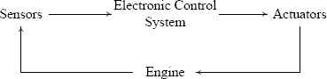
The basic control loop of engine.
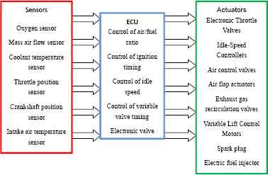
Components of sensors and actuators and basic function of ECU.
2.2. BP neural network
Back propagation (BP) neural network algorithm is a multi-layer feed forward network trained based on an error back propagation algorithm and is one of the most widely applied neural network models. The BP network is used to learn and store a great deal of mapping relations of input-output model. In this network, there is no need to disclose in advance the mathematical equation that describes these mapping relations. Its learning rule is to adopt the steepest descent method in which the back propagation is used to regulate the weight value and threshold value of the network to achieve the minimum error sum of square13. The BP neural network toolbox in Matlab is chosen to get the ideal fault diagnosis results in this study. In order to obtain the best BP neural network structure, a large number of simulation experiments were conducted. Considering the mean squared error and percent error, hidden layer neurons of BP model are confirmed using minimum error and fast calculation speed, so hidden layer neurons are 17. Hidden and output layer incentive functions are purelin and tansig respectively to adjust weight values. The Figure 3 shows the two functions.
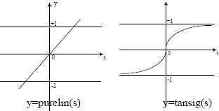
Purelin and tansig function.
The input layer neurons represent input parameters of engine, while the output layer neurons represent faults, so nodes of input and output are confirmed. Table 1 lists the BP neural network model parameters.
| Item name | Content in detail | Parameters |
|---|---|---|
| Neurons node number | Input layer | 10 |
| Hidden Layer | 17 | |
| Output layer | 6 | |
| Network structure function | Input—Hidden layer transfer function | Purelin |
| Hidden—Output layer transfer function | Tansig | |
| Training parameters | Training function | Trainlm |
| Training times | 1000 | |
| Display Interval | 10 | |
| Training goal | 0.001 | |
| Study rate | 0.01 |
BP neural network model parameters.
2.3. Genetic Algorithms(GA)
Genetic Algorithms (GA) are probabilistic search algorithms that emulate the biological evolution of a population, by applying genetic operators that allow the recombination of the individuals, in order to strengthen their performance with regard to a quality function15.
The selection of fitness function directly influences the convergence speed of genetic algorithm and whether it can find the optimal solution. Individual fitness (F) is calculated by Equation 1 .
Where yi is expectation output of node i, and oi is forecast output. k is coefficient, which is a uniform random number rand between 0 and 1. n is an individual number.
2.4. GABP model
Although the BP algorithm is successful, it has some disadvantages. Because the BP neural network has adopted the gradient method, the problems include a slow learning convergent velocity and easy convergence to local minima, which cannot be avoided 14. GA has been proven to effectively function with ANNs in determining the most compact architecture improving the estimation performance in a variety of problems 16. This paper chose GA to optimize BP neural network to avoid BP algorithm convergence to local minima. The weights and thresholds of BP neural network are optimized using GA in training process, so called this algorithm is genetic algorithm BP neural network(GABP). First, we should confirm the original parameters of GA. The population size is set to 10, and the evolution number is 50 times, crossover probability is 0.4, mutation probability is 0.2. Second, confirm fitness function using Equation 1 .
In fitness proportionate individuals are selected with a probability that is directly proportional to their fitness values26. Evaluate the probability, Pi of selecting each individual in the population:
Where N is population size.
Genetic operators are used to evolving the next generation of individuals from the current population 26. Here we choose crossover and mutation. So, next step is crossover and mutation using the equation 3 and 4 17. According to the probability Pi, randomly select two antibodies a and al from the population, then the crossover operation of two antibodies in j-bit can be described as follows:
Where b is a variable randomly distributed from 0 to 1. For the selected antibody ai, the mutation of j-gene can be calculated as follows:
Where amax and amin are the low and upper bounds of the gene value respectively. r is a variable randomly distributed from 0 to 1. Mutation probability is basically a measure of the likeness that random elements of your chromosome will be flipped into something else. For example, if your chromosome is encoded as a binary string of length 100 if you have 1% mutation probability it means that 1 out of your 100 bits (on average) picked at random will be flipped. So f(g) is the mutation probability defined as follows:
Where g is the current iterative number, Gmax is the maximal iterative number, r2 is a variable randomly distributed from 0 to 1.
3. Tests and Experiments
The detection of faults in their early stages is beneficial for the avoidance of larger and more severe faults. Fault detection and diagnosis (FDD) methods are used to monitor the system and identify faults occurring and type and location. If a fault is correctly detected and diagnosed, corrective measures can be applied to repair the fault and reduce any further damage to the system. Many researchers carried out intensive research on FDD18–21. Authors22 used the energy balance equations which balance the relation among pressure, mass flow rate and power at various locations to diagnose the faults of the space shuttle main engine. Authors23 used vibration signals to diagnose the faults of diesel internal combustion engine’s valve trains. Meanwhile, changes of exhaust emissions content reflect engine performance24. Exhaust emissions compositions of engine mainly include HC, NOx, CO, CO2, O2, water vapour etc. They must change in some range due to the change of operating status at different conditions, various mechanical and electronic faults25. So exhaust emissions can reflect engine faults. On the other hand, engine’s sensors data can also reflect engine’s condition and faults. In order to get the comprehensive information of engine to help us diagnose the faults accurately, sensors data27 and emissions information are all used to diagnose the faults of the engine, which are shown in Table 2. Table 2 presents data about the engine, which are called faults feature factors as inputs of the BP neural network and faults type, which are the output of the BP neural network.
| Input item | Feature factors(unit) | Output item | Faults type |
|---|---|---|---|
| x1 | CO(10–2 cc ) | y1 | No fault |
| x2 | CO2(10–2 cc ) | y2 | fuel injector fault |
| x3 | O2(10–2 cc ) | y3 | Ignition coil fault |
| x4 | HC(10–6 cc ) | y4 | Throttle position sensor fault |
| x5 | NOx(10–6 cc ) | y5 | air flow sensor fault |
| x6 | Crankshaft rolling speed(r/min ) | y6 | Oxygen sensor fault |
| x7 | Throttle position(mv) | ||
| x8 | air flow sensor (Hz) | ||
| x9 | Oxygen sensor (mv) | ||
| x10 | Intake air temperature sensor(°C) |
Faults feature factors and faults type.
3.1. Experimental instruments
A test platform is built to verify the proposed method. The platform includes South Korea Hyundai fault test vehicle, X-431 diagnosis instrument and AUTO5-1 exhaust gas analyzer as well as a computer. Figure 4 shows the diagnosis test vehicle, which has eight faults setting control modules. Their names are engine(ECU) faults, ABS(antilock brake system) faults, TCS(Traction Control System), FATC(Full Automatic Air Conditioning), TCU(Transmission Control Unit), ECS(Engine Control System), ETACS(Electronic Time Alarm Control System), Air bag. In this paper, the focus will only be on the engine faults setting module because it has a more direct connection with emissions and system can get the sensors data easily. The engine can be inserted into different sensors faults and actuators faults, then diagnose the inserted faults using the proposed method and get the diagnosis results. Comparing diagnosis results with the inserted faults, which can test the diagnostic system.
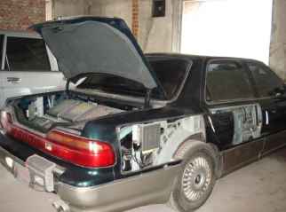
Diagnosis test vehicle.
The X-431 diagnosis instrument is shown in Figure 5, which can get sensors data flow. Figure 6 shows the AUTO5-1 exhausts gas analyzer, which can get exhaust information of engine. The vehicle only runs at the idle condition, because we need to connect the experiment instruments with the vehicle and get the information. In order to simulate real road conditions, we use Burke Porter’s 3600 roll brake test system. Figure 7 shows the vehicle running on the platform. We can get the vehicle’s information on different speed and diagnose the faults real-time (on-line).
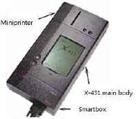
The main body appearance of X-431.
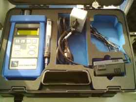
AUTO5-1 exhausts gas analyzer.
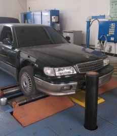
Vehicle running on the 3600 roll brake test systems.
3.2. Experiment data acquisition
It should be noted that the use of artificial neural networks requires the collection of large amounts of data sets. They require obtaining more than one hundred sets of data for each operating condition, which are used to teach the network. We use the diagnostic port MITSUBISHI/HYUNDAI-12+16. The 16 frame port is standard RS232. Sensors data flow can be got using X-431 PCLINK data communication soft, which can realize the following functions shown in table 3. Figure 8 represents the software main interface.
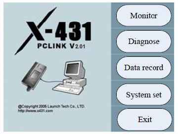
Main interface of PCLINK diagnosis software.
| Functions | Explanation |
|---|---|
| Monitor and alarm | monitor the engine and give the alarm if the engine has abnormal. |
| Diagnose | diagnose the faults of the engine. |
| Restore and check | restore and check data of engine such as speed, coolant temperature and so on. |
| Reset system | reset system such as deleting fault code, recovering system etc. |
PCLINk data communication soft functions.
The test vehicle and all the instruments can work normally before doing experiments in order to get the right information about the engine. Faults’ code must be cleared on the X-431 diagnostic instrument and the AUTO5-1 exhaust gas analyzer must be reset. All of the fault set modules of test vehicle must keep normal. We must keep the X-431 and the AUTO5-1 to work together, which can ensure we get the information on same time. Firstly, the vehicle runs at idle speed, and then it keeps running at this condition and gets the normal data. Parts of normal and different faults data engine at idle speed are shown in Table 4. Secondly, vehicle will accelerate until 1800r/min, and then the vehicle keeps running at this speed and gets the normal data. Parts of normal data and different faults data engine at 1800r/min are shown in table 5. We performed these steps 20 times and got 120 groups data.
| Fault type | x1 | x2 | x3 | x4 | x5 |
|---|---|---|---|---|---|
| y1 | 0.01 | 9.1 | 4.43 | 1 | 431 |
| y1 | 0.01 | 12.7 | 3.38 | 1 | 664 |
| y2 | 0.07 | 7.8 | 10.82 | 1532 | 91 |
| y2 | 0.08 | 7.8 | 10.81 | 1534 | 95 |
| y3 | 0.01 | 10 | 9.32 | 1 | 984 |
| y3 | 0.02 | 9.3 | 9.7 | 1 | 1008 |
| y4 | 0.17 | 8.9 | 8.7 | 1344 | 38 |
| y4 | 0.16 | 9.2 | 8.57 | 1344 | 44 |
| y5 | 0.11 | 10.3 | 4.98 | 1543 | 89 |
| y5 | 0.12 | 10.4 | 4.93 | 1543 | 92 |
| y6 | 0.06 | 8.7 | 8.76 | 883 | 30 |
| y6 | 0.07 | 9.1 | 8.52 | 915 | 31 |
| Fault type | x6 | x7 | x8 | x9 | x10 |
| y1 | 718.8 | 507.8 | 23.1 | 39.1 | 17 |
| y1 | 687.5 | 507.8 | 23.1 | 39.1 | 17 |
| y2 | 718.8 | 507.8 | 31.2 | 58.6 | 16 |
| y2 | 687.5 | 507.8 | 31.2 | 58.6 | 16 |
| y3 | 718.8 | 507.8 | 43.8 | 39.1 | 17 |
| y3 | 687.5 | 507.8 | 43.8 | 39.1 | 17 |
| y4 | 718.8 | 19.5 | 37.5 | 58.6 | 19 |
| y4 | 687.5 | 19.5 | 31.2 | 58.6 | 19 |
| y5 | 718.8 | 507.8 | 0 | 273.4 | 17 |
| y5 | 687.5 | 507.8 | 0 | 293 | 17 |
| y6 | 718.8 | 507.8 | 37.5 | 19.5 | 16 |
| y6 | 687.5 | 507.8 | 37.5 | 19.5 | 16 |
Note: x1-CO, x2- CO2 x3- O2, x4- HC, x5- NOx x6- engine speed, x7- position of throttle valve, x8- air flow rate, x9-oxygen sensor, x10- air temperature sensor;
y1-normal, y2- nozzle fault, y3-ignition coil fault, y4- throttle valve sensor fault, y5- air flow sensor fault, y6-oxygen sensor fault
Training data engine at idle speed.
| Fault type | x1 | x2 | x3 | x4 | x5 |
|---|---|---|---|---|---|
| y1 | 0 | 13.5 | 2.99 | 46 | 1397 |
| y1 | 0 | 13.5 | 2.93 | 47 | 1590 |
| y2 | 0 | 11.6 | 3.78 | 1 | 1115 |
| y2 | 0 | 11.2 | 3.52 | 1 | 1487 |
| y3 | 0.04 | 9.3 | 8.63 | 1 | 1228 |
| y3 | 0.06 | 9.4 | 8.59 | 1 | 1215 |
| y4 | 0.01 | 13.8 | 2.28 | 1 | 1412 |
| y4 | 0.01 | 13.8 | 2.52 | 1 | 1027 |
| y5 | 0.79 | 14.9 | 0.41 | 322 | 143 |
| y5 | 0.84 | 14.9 | 0.4 | 356 | 133 |
| y6 | 0.01 | 13.9 | 2.39 | 1 | 1675 |
| y6 | 0.01 | 13.5 | 2.58 | 1 | 1916 |
| Fault type | x6 | x7 | x8 | x9 | x10 |
| y1 | 1875 | 957 | 156.2 | 58.6 | 54 |
| y1 | 1812.5 | 937.4 | 150 | 58.6 | 54 |
| y2 | 1875 | 1074.2 | 187.5 | 39.1 | 32 |
| y2 | 1812.5 | 1054.6 | 181.2 | 39.1 | 32 |
| y3 | 1875 | 2382.7 | 368.8 | 39.1 | 0 |
| y3 | 1812.5 | 2382.7 | 406.2 | 39.1 | 0 |
| y4 | 1718.8 | 39.1 | 150 | 39.1 | 0 |
| y4 | 1812.5 | 39.1 | 156.2 | 58.6 | 0 |
| y5 | 1875 | 917.9 | 0 | 917.9 | 54 |
| y5 | 1812.5 | 937.4 | 0 | 937.4 | 54 |
| y6 | 1781.2 | 937.4 | 156.2 | 39.1 | 32 |
| y6 | 1718. 8 | 839.8 | 156.2 | 19.5 | 32 |
Training data of engine accelerate to 1800r/min
4. Algorithm model training
4.1. BP Neural network training
BP neural network model is built using Matlab software and trained using the data. Figure 9 shows the training interface, which gives the structure of the neural network, algorithms parameters, calculates progress and training plots. Figure 10 presents change curve of BP neural network training mean squared error with training epochs. From Figure 10(a) we can see the best validation performance is 1.49 × 10⁻⁵ at epoch 13, which mean the neural network convergence speed is very fast. Figure 11 shows the BP neural network training objective gradient curve, while Figure 12 shows the linear correlation-regression curve of a relative output of the BP neural network. The training curves of the engine are provided using different data at the idle speed and accelerate to 1800r/min respectively.
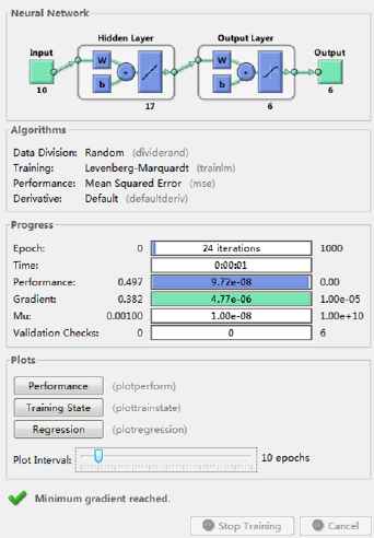
Neural network training interface.
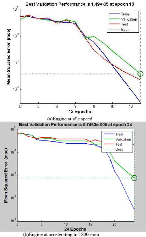
The change curve of BP neural network training mean squared error with the training epoch.
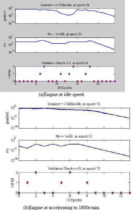
BP neural network training objective gradient curve.
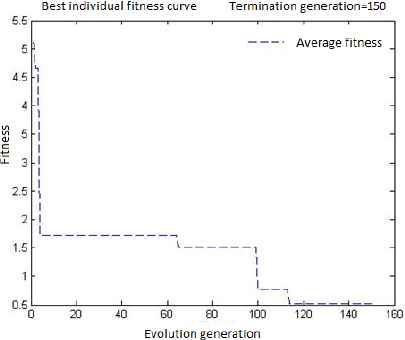
Best individual fitness curve.
Figure 11 shows that neural network model is trained to 24 epochs by iteration, and the declining gradient can reach required minimum. Target error is in the minimum range, which can illustrate that training of neural network model is ideal. It can meet convergence requirement. It can reach the minimum gradient 1e-005 and the minimum target error less than 0.001, which illustrate that the model can change and confirm the weights that link different layers. Figure 11(a) shows that best validation performance is 5.7463e-005 at epoch 24.
4.2. GABP training
The best individual fitness curve and best fitness were obtained by training (showing in Figure 12). The steps of convergence GABP neural network model is shown in Figure 13.

Process of GABP network training.
As it can be seen from Figure 12, the best individual fitness curve stabilizes after 110 generations, which indicates that the best individual has been achieved optimizing network to 110 generations. Comparing the same structure pure BP neural network, the GABP can improve the performance of the neural network, but it also increases the training convergence time.
4.3. Test on line
We test faults diagnosis on line using the model, which has been trained BP neural network. Table 6 provides a group of data engine accelerate to 1800r/min. The data have been normalized. The normalized calculated method is shown as follows:
| x1 | x2 | x3 | x4 | x5 | |
|---|---|---|---|---|---|
| 1 | 0.0000 | 0.0045 | 0.0012 | 0.0201 | 0.9452 |
| 2 | 0.0000 | 0.0038 | 0.0020 | 0.0000 | 0.7373 |
| 3 | 0.0001 | 0.0034 | 0.0028 | 0.0003 | 0.3983 |
| 4 | 0.0000 | 0.0048 | 0.0012 | 0.0003 | 0.4038 |
| 5 | 0.0007 | 0.0050 | 0.0001 | 0.3175 | 0.0180 |
| 6 | 0.0000 | 0.0045 | 0.0012 | 0.0003 | 1.0000 |
| x6 | x7 | x8 | x9 | x10 | |
| 1 | 0.6282 | 0.3182 | 0.0520 | 0.0203 | 0.0187 |
| 2 | 0.6282 | 0.3520 | 0.0650 | 0.0136 | 0.1109 |
| 3 | 0.6282 | 0.8860 | 0.1538 | 0.0136 | 0.0000 |
| 4 | 0.6282 | 0.0136 | 0.0520 | 0.0203 | 0.0000 |
| 5 | 0.6282 | 0.3317 | 0.0000 | 0.3114 | 0.0187 |
| 6 | 0.6282 | 0.3182 | 0.0520 | 0.0068 | 0.1109 |
A group of test data.
Within a given bounded data set there is often a large difference between the maximum and the minimum values. When normalization is applied to a data set its’ upper and lower bounds are scaled to appreciably smaller magnitudes. We use the basic z-score normalization that is obtained by using Equation 6
Where μ (x) and σ (x) denote the normal data and the standard deviation of x, respectively. This normalization produces a data set, where each point has a normal close to zero and a variance close to one.
Figure 14 provides the parameters curve when the Oxygen sensor fault is set. Table 7 provides diagnosis results of test data. It can be seen that the real output of the neural network is close to the expected output.
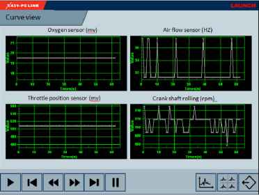
Parameters curves when oxygen sensor has a fault.
| Sample | BP neural network real output | Expected output | |||||
|---|---|---|---|---|---|---|---|
| 1 | 0.9886 | 0.1143 | 0.0707 | 0.0090 | 0.0903 | 0.0607 | (100000)’ |
| 2 | 0.0986 | 0.9790 | 0.0789 | 0.0924 | 0.1022 | 0.0968 | (010000)’ |
| 3 | 0.1018 | 0.1015 | 0.9408 | 0.1027 | 0.1428 | 0.1118 | (001000)’ |
| 4 | 0.1193 | 0.0996 | 0.1175 | 0.9471 | 0.0732 | 0.0854 | (000100)’ |
| 5 | 0.0617 | 0.0862 | 0.1401 | 0.0810 | 0.9181 | 0.0838 | (000010)’ |
| 6 | 0.0444 | 0.1025 | 0.0132 | 0.0429 | 0.0001 | 0.9327 | (000001)’ |
Diagnosis results.
5. Discussions
We used X-431 to get the test vehicle’s sensors data and used the AUTO5-1 exhaust gas analyzer to get the emissions information. These data were sent to BP neural network and GABP model to train the two models then using the trained model to diagnose faults.
We test 120 groups of data, which can be diagnosed are 118 groups of data. The accuracy of diagnosis can reach 98.33%. If only use sensors data flow and exhaust emissions information the accuracy of diagnosis is 93.33 and 83.33% respectively. It means that we use sensors data flow and exhaust emissions information to diagnose engine’s faults is valid and better than only use one.
We also diagnosed these data using GABP model, it can diagnose all faults accurately and the precision is higher than BP neural network, but training convergence time is increased.
It is must be pointed that we cannot guarantee the exhaust emission information keep up with the sensor data flow because they are collected using different equipment. X-431 gets the engine sensors data and then sends the data to the computer. AUTO5-1 exhaust gas analyzer gets the exhaust gas information and then sends the information to the computer. There is no connection between the two devices. They send information independently, so we cannot insure that they can get the engine’s information at the same time. How can we get synchronous data is needed to research deeply. The model should be modified further for raising the accuracy of fault diagnosis on the other hand.
6. Acknowledgement
This work is supported by the Fundamental Research Funds for the Central Universities (NO.2572018BG02).
References
Cite this article
TY  - JOUR
AU  - Chunli XIE
AU  - Yuchao Wang
AU  - John MacIntyre
AU  - Muhammad Sheikh
AU  - Mustafa Elkady
PY  - 2018
DA  - 2018/06/04
TI  - Using Sensors Data and Emissions Information to Diagnose Engine’s Faults
JO  - International Journal of Computational Intelligence Systems
SP  - 1142
EP  - 1152
VL  - 11
IS  - 1
SN  - 1875-6883
UR  - https://doi.org/10.2991/ijcis.11.1.86
DO  - 10.2991/ijcis.11.1.86
ID  - XIE2018
ER  -