
Optimization of quality measures in association rule mining: an empirical study
- DOI
- 10.2991/ijcis.2018.25905182How to use a DOI?
- Keywords
- Quality measures; Association rule mining; Optimization; Empirical study
- Abstract
In the association rule mining field many different quality measures have been proposed over time with the aim of quantifying the interestingness of each discovered rule. In evolutionary computation, many of these metrics have been used as functions to be optimized, but the selection of a set of suitable quality measures for each specific problem is not a trivial task. The aim of this paper is to review the most widely used quality measures, analyze their properties from an empirical standpoint and, as a result, ease the process of selecting a subset of them for tackling the task of mining association rules through evolutionary computation. The experimental analysis includes twenty metrics, thirty datasets and a diverse set of algorithms to describe which quality measures are related (or unrelated) so they should (or should not) be used at time. A series of recomendations are therefore provided according to which quality measures are easily optimized, what set of measures should be used to optimize the whole set of metrics, or which measures are hardly optimized by any other.
- Copyright
- © 2018, the Authors. Published by Atlantis Press.
- Open Access
- This is an open access article under the CC BY-NC license (http://creativecommons.org/licences/by-nc/4.0/).
1. Introduction
The discovery of valuable and unknown information from big amounts of data gathered from different domains is essential for many companies that aim to take any advantage of that17. This information may be defined under the term pattern24, which represents any type of homogeneity and regularity in data, providing intrinsic and important properties of them1. Association rules were proposed at the beginning of the nineties2 as a way of describing associations among patterns so more descriptive analysis can be achieved. These associations are implications of the form X → Y, X and Y being patterns with no common item (X ∩Y = ∅) whose meaning is that one of the sets leads to the presence of the other set26.
Generally, existing algorithms for mining association rules produce a huge output that hampers the process of analysing the utility and interest of the results. In this regard, interestingness quality measures can be used to filter and/or rank the output, producing a reduced set of association rules easily understandable. These quality measures are divided into objective and subjective metrics. Objective measures are said to be data-driven and only take into account statistical and structural properties of data22, serving as a filter to select interesting patterns/associations. On the contrary, subjective measures are user-driven in the sense that they take into account the user’s preferences and goals. This user is not assumed to be a data mining expert, but rather an expert in the field being analysed.
Different models7 have been proposed over time to produce a comprehensible and reduced set of rules that improve the clarity of the output. In this sense, evolutionary algorithms24 have achieved excellent results due to their ability to look for optimal solutions according to a single or a set of quality measures. Some additional studies based on evolutionary computation aimed at combining a set of quality measures by assigning different weights to each one16 or by finding good compromises among them14,20. At this point and even when many existing models are conducted at using different quality measures on different ways, it is still hard to find a general and unbiased study that helps users in finding which measure (or pair of them) should be used. The aim of this paper is therefore to review the most widely used quality measures, describing and analyzing their properties, and providing the reader with a general knowledge of their behaviour to ease the process of selecting one or more measures when tackling an association rule mining problem. The strong point of this paper is the empirical analysis carried out, including twenty metrics, thirty datasets, and a diverse set of evolutionary algorithms that optimize a single measure12,13,15,20,25 or multiple metrics at time6,27. An exhaustive search approach9 is also considered to validate the degree of optimization achieved by the evolutionary algorithms. The final aim of this experimental analysis is to describe which quality measures are related (or unrelated) so they should (or should not) be used at time.
Results obtained in the experimental study provide a series of recomendations according to which quality measures are easily optimized, what set of measures should be used to optimize the whole set of metrics, or which measures are hardly optimized by any other. This information is essential for any researcher in the design of an optimal evolutionary algorithm for mining association rules. As an example of knowledge extracted by this analysis, it is described that any algorithm that considers Support/Confidence as measures to be optimized should avoid a set of metrics (Coverage, Prevalence, CF, Laplace, ECR and Zhang) since they are also optimized at time. It provides a really useful infomation since there is no sense to choose any of the aforementioned metrics when Support/Confidence are being optimized. It is our understanding that the knowledge provided in this study is of high interest for future researches on the field, determining which quality measures are more general and which one (or pair of them) should be used if other different metrics are required to be optimized.
The remainder of the paper is as follows. Section 2 overviews the most relevant quality measures used in association rule mining, providing formal definitions (Section 2.1), analysing the general properties for any quality measure (Section 2.2), and determining how the most widely used quality measures are related (Section 2.3). Section 3 provides an extensive experimental study about the behaviour of a set of twenty quality measures and considering thirty datasets. Finally, Section 4 summarizes the conclusions drawn from the conducted analysis.
2. Quality measures
The aim of this section is to serve as a preliminar analysis, providing a general overview of the most well-known quality measures in association rule mining. In this regard, some formal definitions for the existing quality measures are first introduced. Then, some general properties that should satisfy any good quality measure are described. Finally, the two most widespread metrics (Support and Confidence) in the association rule mining field are mathematically analysed, describing how they are related to the most widely used quality measures.
2.1. Formal definitions
The mining of valuable and previously unknown association rules in a database might produce a large amount of different solutions, giving rise to a hard process of analysing each single rule. Besides, a large percentage of this set of solutions may be uninteresting and useless, being the user responsible for reducing the output by means of a process of quantifying the association rules24. To solve this issue, different quality measures (see Table 1) based on the analysis of the statistical properties of data have been proposed by different authors4,21.
| Name | Equation | Feasible values |
|---|---|---|
| Support | pxy | [0, 1] |
| Coverage | px | [0, 1] |
| Prevalence | py | [0, 1] |
| Confidence |
|
[0, 1] |
| Lift |
|
[0, n] |
| Cosine |
|
[0, 1] |
| Leverage | pxy − (px × py) | [-0.25, 0.25] |
| Conviction |
|
|
| CC |
|
|
| CF |
|
[-1, 1] |
| Recall |
|
[0, 1] |
| Laplace |
|
|
| Pearson |
|
|
| IG |
|
|
| Sebag |
|
[0, n − 1] |
| LC |
|
|
| ECR |
|
[2 − n, 1] |
| Zhang |
|
[-1, 1] |
| Netconf |
|
[-1, 1] |
| Yule’sQ |
|
[-1, 1] |
Quality measures and range of feasible values.
The principal element in association rule mining is the pattern P, which is defined as a subset of the whole set of items I = {i1,i2,…,il} in a dataset Ω, i.e. P = {ij,…,ik} ⊆ I, 1 ≤ j,k ≤ l. An association rule is an implication of the form X → Y that is formed from P in such a way that the antecedent X is defined as X ⊂ P, whereas the consequent Y is denoted as Y = P \ X. Any existing quality measure in this field is based on the number of transactions in the dataset satisfied by the rule (denoted as nxy), the antecedent (nx), and the consequent (ny). All these values (nxy, nx and ny) can also be represented as relative frequencies, by considering the number n of transactions in data, in per unit basis:
pxy = nxy/n; pxӯ = nxӯ/n;
Support2 is the most well-known quality measure in association rule mining. It is defined as the relative frequency of occurrence of an association rule X → Y, i.e. Support(X → Y) ≡ pxy. Symmetry is a major feature of this quality measure, i.e. Support(X → Y) = Support(Y → X), so it does not quantify any implication between the antecedent X and the consequent Y. Additionally, the minimum and maximum values for this quality measure are 0 and 1, respectively. However, an association rule is considered as misleading if one of these two values is obtained. Thus, in situations where pxy = 1, then the rule is useless since it appears in any transaction so it does not provide any new knowledge about the data properties. On the contrary, if pxy = 0, then the rule does not represent any transaction so it is considered as misleading. This last situation might be caused by the two following issues: (a) px = 0 or py = 0, so both X and Y do not have any transaction satisfied in common; (b) either the antecedent X and the consequent Y satisfy up to 50% of the transactions within the dataset, i.e. px ≤ 0.5 and py ≤ 0.5, but they do not satisfy any transaction in common. An important property of the Support quality measure is that it is always greater than 0 when px + py > 1, and its maximum value is always equal to the minimum value among px and py, i.e. pxy ≤ Min{px, py}.
Coverage and Prevalence21 quality measures are defined as the Support on the basis of the antecedent X or the consequent Y, respectively. Coverage, defined as px, determines the percentage of transactions where the antecedent X appears. On the contrary, the Prevalence quality measure, i.e. py, determines the percentage of transactions where the consequent Y appears. It is noteworthy that, similarly to Support, these two quality measures operate in the range [0,1].
Confidence is a quality measure that appears in most of the problems where the mining of association between patterns is a dare26. This quality quality measure is defined as the percentage of transactions in a dataset containing X and, at the same time, also Y. In a formal way, this quality measure can be expressed as Confidence(X → Y) = pxy/px, or as an estimate of the conditional probability P(Y|X). It should be highlight that Confidence quality measure operates on the interval [0,1] and it is not symmetric, i.e. Confidence(X → Y) ≠ Confidence(Y → X), denoting implication between X and Y. However, it is possible to obtain that Confidence(X → Y) = Confidence(Y → X) in situations where px = py regardless the pxy value.
Lift (also called interest)5 is one of the many alternative quality measures proposed by different authors. This quality measure calculates the relationship between the Confidence of the rule and its Prevalence. As shown in Table 1, Lift quality measure is described as Lift(X → Y)= pxy/(px × py), or also as Lift(X → Y) = Confidence(X → Y)/py. This measure calculates a ratio between the joint probability of two observing variables (antecedent X and consequent Y) with respect to their probabilities under the independence assumption. Lift may produce invalid results when px or py is equal to 0, i.e. Lift(X → Y) = 0/0. Otherwise, Lift is defined within the range [0,n] and it is symmetric. The minimum value is obtained when pxy = 0 and px ≠ 0 and/or py ≠ 0, whereas the maximum value is obtained when pxy = px = py = 1/n (only one transaction is satisfied within the dataset). This measure may also be defined as a correlation measure, calculating the degree of dependence between the antecedent and consequent of a rule. Lift values lower than 1 determine a negative dependence (positive dependence for values greater than 1), whereas a value of 1 stands for independence.
Cosine (also called IS)21 is a quality metric derived from Lift. Cosine is formally defined as
Leverage was proposed by Piatetsky-Shapiro19 as a quality measure quite similar to Lift. Leverage determines how different is the co-occurrence of the antecedent X and the consequent Y of a rule from independence10. This quality measure, also known as novelty3, is formally defined as Leverage(X → Y)=pxy − (px × py), and it takes values in the range [−0.25,0.25], denoting a zero value in those cases where the antecedent X and consequent Y are statistically independent. Finally, similarly to Support, Lift and Cosine quality measures, Leverage also includes symmetry as an important property, i.e. Leverage(X → Y) = Leverage(Y → X).
Conviction5 was proposed as a way of representing the degree of implication of a rule, and values far from the unity indicate interesting rules. This quality measure (see Table 1) is formally defined as Conviction(X → Y)=(px × pӯ)/pxӯ, which can also be defined as Conviction(X → Y)=(px − (px × py))/(px − pxy). Conviction takes values in the range [1/n,n/4]. Whereas lower bound is reached when px = pӯ = pxӯ since px = 0 produces an indetermination, the upper bound is reached when px = pӯ = 0.5 and pxӯ = 1/n.
Centered Confidence (CC)10, also called relative accuracy or gain is formally defined as gain(X → Y) = Confidence(X → Y) − py). As shown in Table 1, the centered Confidence measure produces values in the range [−1,1 − 1/n], being impossible to produce a value equal to unity. Note that the maximum feasible value is achieve when py is minimum and Confidence(X → Y) is maximum. The minimum feasible value of py is py = 1/n since 0 values does not produce maximum Confidence values, i.e. py = 0 = pxy so Confidence(X → Y) = 0. Hence, the maximum value for the centered Confidence or gain is equal to gain(X → Y) = 1 − 1/n, when pxy = px and py = 1/n.
Other quality measures have been proposed by many authors as interesting quality measures to be considered. Even when almost all the existing works in the association rule mining field include, at least, one of the aforementioned quality measures, there are many other additional measures that might be used in different scenarios (see Table 1) including the following: certainty factor (CF)4 is defined as the gain normalized into the interval [−1,1], i.e. CF(X → Y) = gain(X → Y)/pӯ if gain(X → Y) ≥ 0), and CF(X → Y) = gain(X → Y)/py if gain(X → Y) < 0); Recall8 (Recall(X → Y) = pxy/py) is denoted as the percentage of transactions in a database containing Y and, at the same time, also X; Laplace measure8 is formally stated as Laplace(X → Y) = (nxy + 1)/(nx + 2) and it can be transformed to (pxy × n + 1)/(px × n + 2); pearson’s correlation coefficient11, which is defined as
2.2. Properties of quality measures
As previously described, many objective quality measures have been proposed in the literature to quantify the interest of the knowledge extracted. The analysis of these measures is not trivial and many different and opposed properties have been considered by different researchers, denoting that these properties can be divided into two main different sets, i.e. the one proposed by Piatetsky-Shapiro19 and the one of Tan et al.22.
Piatetsky-Shapiro19 suggested that any quality measure ℳ defined to quantify the interest of an association rule should verify three specific properties in order to separate strong and weak rules so high and low values can be assigned, respectively. These properties are described below and Table 2 summarizes which quality measure satisfies each of the three properties. The first property (P1) states that an association rule which occurs by chance has zero interest value, that is, it is not interesting. P1 claims that any quality measure ℳ should test whether X and Y are statistically independent, denoting that ℳ (X → Y) should be 0 when pxy = px × py. Property number two (P2) states that the greater the Support, the greater the interestingness value when the Support for X and Y is fixed, that is, the more positive correlation X and Y have, the more interesting the rule. Here, ℳ (X → Y) monotonically increases with pxy when px and py remain the same. The third property (P3) states that if the Supports for the rule and Y (or X) are fixed, the smaller the Support for X (or Y), the more interesting the pattern. Considering P3, ℳ (X → Y) monotonically decreases with px or with py when other parameters remain the same, i.e. pxy and px or py remain unchanged.
| Piatetsky-Shapiro19 | Tan et al.22 | |||||||
|---|---|---|---|---|---|---|---|---|
| Measure | P1 | P2 | P3 | O1 | O2 | O3 | O4 | O5 |
| Support | No | Yes | No | Yes | No | No | No | No |
| Coverage | No | No | No | No | No | No | No | No |
| Prevalence | No | No | No | No | No | No | No | No |
| Confidence | No | Yes | No | No | No | No | No | Yes |
| Lift | No | Yes | Yes | Yes | No | No | No | No |
| Cosine | No | Yes | Yes | Yes | No | No | No | Yes |
| Leverage | Yes | Yes | Yes | Yes | No | Yes | Yes | No |
| Conviction | No | Yes | No | No | No | No | Yes | No |
| CC | Yes | Yes | Yes | No | No | No | No | No |
| CF | Yes | Yes | Yes | No | No | No | Yes | No |
| Recall | No | Yes | No | No | No | No | No | No |
| Laplace | No | Yes | No | No | No | No | No | No |
| Pearson | Yes | Yes | Yes | Yes | No | Yes | Yes | No |
| IG | Yes | Yes | Yes | Yes | No | No | No | Yes |
| Sebag | No | Yes | Yes | No | No | No | No | Yes |
| LC | No | Yes | Yes | No | No | No | No | Yes |
| ECR | No | Yes | Yes | No | No | No | No | Yes |
| Zhang | Yes | No | No | No | No | No | No | No |
| Netconf | No | Yes | Yes | No | No | No | No | Yes |
| Yule’sQ | Yes | Yes | Yes | Yes | Yes | Yes | Yes | No |
Summary of properties satisfied by a set of different objective quality measures.
Tan et al.22 proposed a different set of properties based on operations for 2x2 contingency tables. The five proposed properties are described below and all the aforementioned quality measures have been tested regarding these five properties (see Table 2). The first property (O1) is related to the symmetry under variable permutation. In this sense, a measure ℳ satisfies this property if and only if ℳ (X → Y) = ℳ (Y → X). The second property (O2) determines invariance when we scale any row or column by a positive factor. Property number three (O3) describes the antisymmetry under row/column permutation. A normalized measure ℳ is antisymmetric under the row permutation operation if ℳ (TR)=-ℳ (T), considering T as the table of frequencies and TR as the table of frequencies with a permutation on the rows; whereas the measure ℳ is antisymmetric under the column permutation operation if ℳ (TC)=-ℳ (T), considering TC as the table of frequencies with a permutation on the columns. According to the authors22 measures that are symmetric under the row and column permutation operations do not distinguish well between positive and negative correlations so it should be careful when using them to evaluate the interestingness of a pattern. Analysing the O3 property, it is stated that ℳ (X → Y) = −ℳ (X → ¬Y) = −ℳ (¬X → Y), so it means that the measure can identify both positive and negative correlations. Property O4 states that ℳ (X → Y) = ℳ (¬X → ¬Y), so property O3 is in fact a special case of this one, i.e. O4. Note that when permuting the rows (columns) causes the sign to change once and permuting the columns (rows) causes it to change again, so the overall result of permuting both rows and columns will be to leave the sign unchanged. The fifth property (O5) states that the measure ℳ should only take into account the number of records containing X, Y, or both. O5 is a null invariance property, denoting that if we change just the values of
As a summary, Table 2 shows that there are six quality measures (Leverage, centered Confidence, certainty factor, pearson, information gain and yule’sQ) that satisfy the three properties proposed by Piatetsky-Shapiro19. According to the set of properties provided by Tan et al.22 there are three measures (Leverage, pearson and yule’sQ) that satisfy a higher number of properties. However, it is noteworthy that not all the properties are required to be satisfied. For instance, in association rule mining, it is of high interest to determine the implication, not the co-occurrence, so property O1 is not desirable. Note that a measure ℳ satisfies O1 if and only if ℳ (X → Y) = ℳ (Y → X). Hence, even when Leverage quality measure seems to be a really good metric (it satisfies almost all the properties), it does not provide implication (Leverage(X → Y) = Leverage(Y → X)) so it should be used together with other quality measure18 that provide implication (O1 property should not be satisfied), e.g. Confidence.
2.3. Relationships between the most well-known quality measures
The analysis of existing quality measures, which score the interest of any association rule, is cornerstone to ease the process of choosing the right metric. In this regard, many different quality measures have been proposed along the years, but the simultaneous optimization of all measures is complex and might lead to poor results. The selection of which quality measure should be optimized is of high importance, determining which kind of rules will be extracted. Additionally, to analyse the existing relationships among measures is essential since the maximization of a specific measure could imply the optimization of many more in the best case scenario. With this aim, and considering Support and Confidence as the basic pillars of any good quality measure2, it is of high interest to mathematically describe the relationship between different metrics and Support/Confidence. Here, the most widespread quality measures (Support, Confidence, Lift, Cosine, Leverage and Conviction) in the association rule mining field24 are considered.
Support/Confidence.
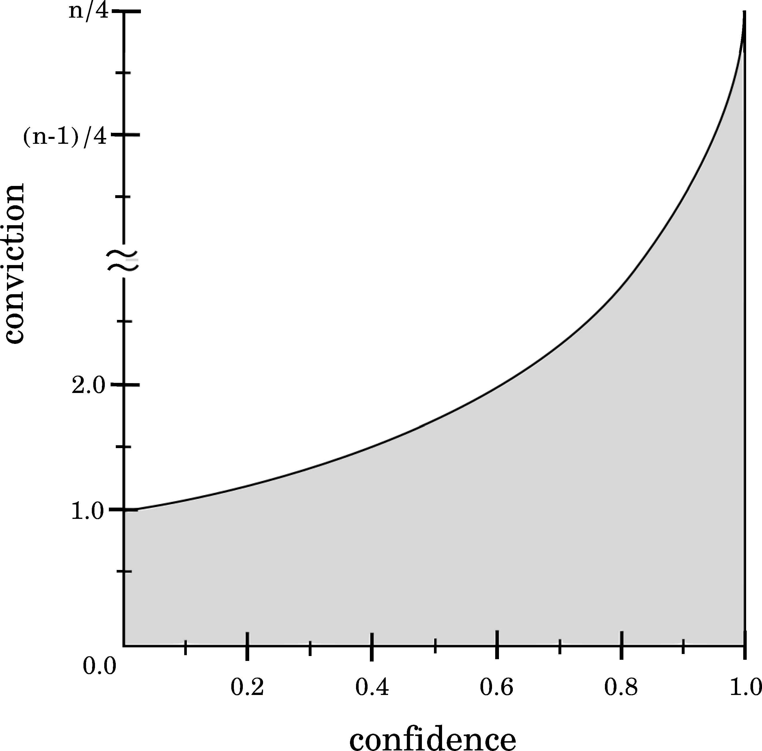
First, it is appealing to determine the existing relationship between Support and Confidence quality measures (see Figure 1). Note that the shaded region illustrates the feasible area in which any association rule can obtain the values. In order to understand the aforementioned relationship, it should be noted that pxy ≤ Min{px, py}, and pxy ≤ px. Thus, given a value pxy, then px will have a value in the range px ∈ [pxy, 1].
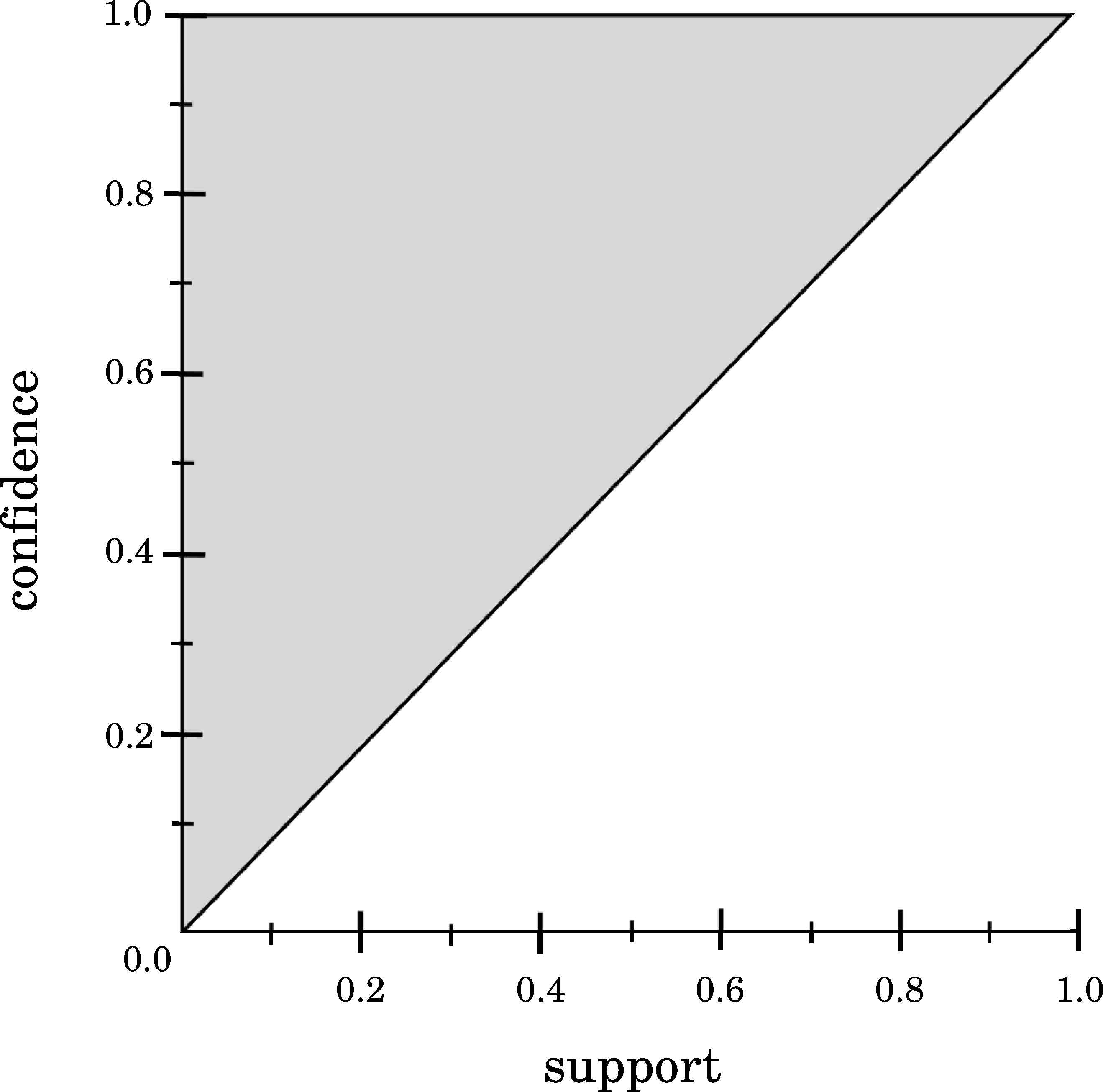
Relationship between Support and Confidence.
According to the previous information, pxy/px ≥ pxy so it is possible to assert that Confidence(X → Y) is always greater or equal to Support(X → Y). As shown in Figure 1, it is not possible to obtain a high Support value and a low Confidence value at the same time, and this information is essential to be known beforehand. Hence, this analysis reveals that a high co-occurrence (high values of pxy) implies a high implication (high values of pxy/px), whereas a high implication does not imply a high co-occurrence.
Lift vs Support/Confidence.
As it is illustrated in Figure 2, for any Support value pxy and considering Lift values lower than unity, then Lift increases when Support also does. On the contrary, when considering Lift values greater than unity, then Lift increases when Support decreases. In fact, high Support values tend to produce Lift values around unity, implying an independence between antecedent and consequent of the rule. Finally, it should be noted that Support values equal to unity implies Lift values close to unity, but the opposite is not necessarily true. This information is essential to be known in advance, so any user or expert knows that it is not possible to optimize both Support and Lift (high values) at time.
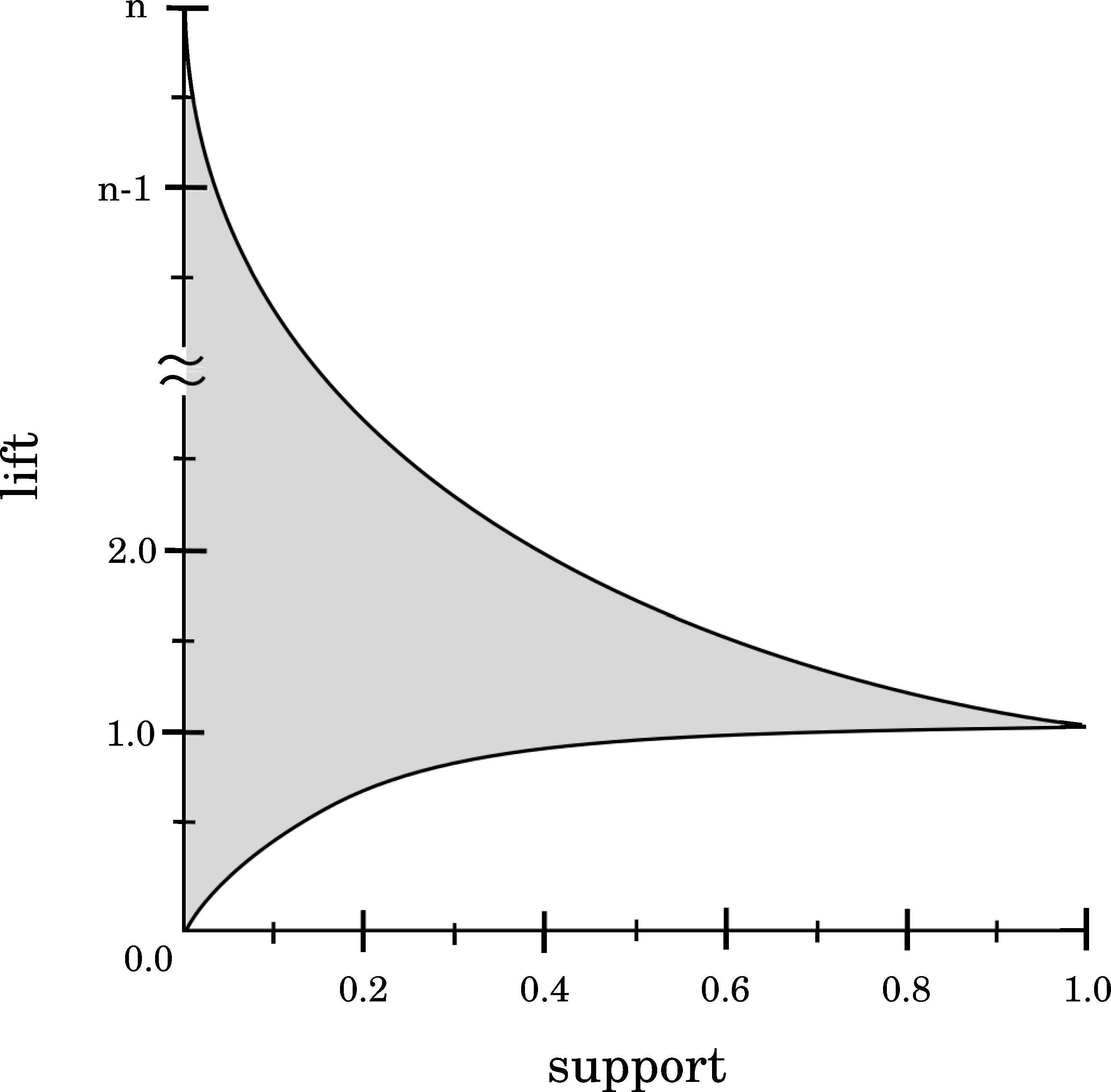
Relationship between Lift and Support.
Analysing the existing relationship between Confidence (pxy/px) and Lift (pxy/(px × py)), it is possible to define Lift on the basis of Confidence as Lift(X → Y)= Confidence(X → Y)/py. Lift quality measure produces maximum values when py is minimum, i.e. py = 1/n, so the maximum values for this quality measure is obtained as Liftmax(X → Y)= Confidence(X → Y) × n. On the contrary, Lift produces minimum values when py is maximum, i.e. py = 1, so the minimum values for Lift quality measure is obtained as Liftmax(X → Y)= Confidence(X → Y). This relationship is shown in Figure 3. As it is illustrated, for maximum Confidence values, i.e. Confidence(X → Y) = 1, then the Lift value will be in the range [1,n]. This analysis reveals that low Confidence values produce low Lift values (lower than unity), denoting a negative correlation. On the contrary, it is easy to obtain a positive correlation (positive Lift values) when Confidence produces high values (close to unity).
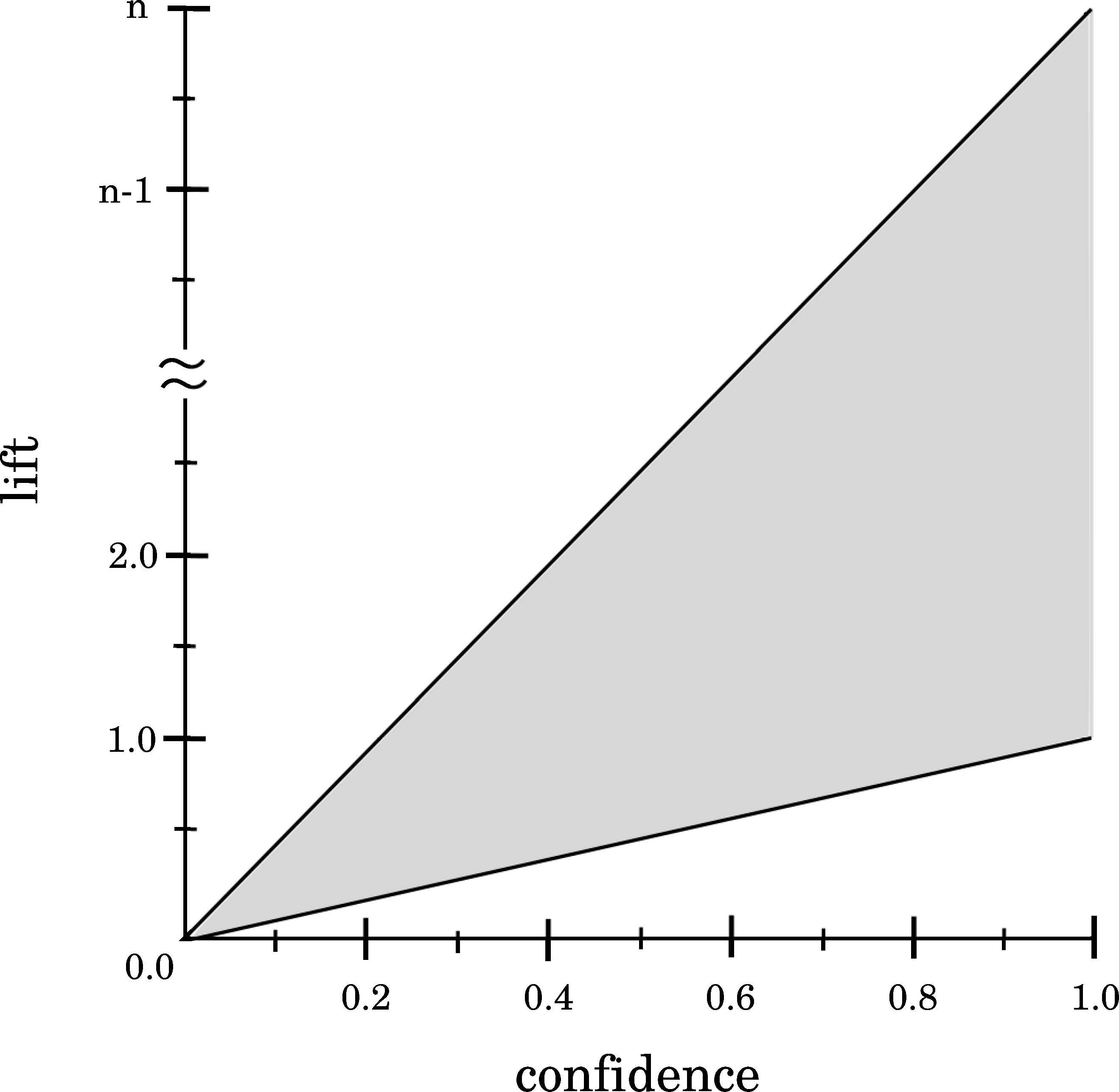
Relationship between Lift and Confidence.
Cosine vs Cupport/Confidence.
Comparing Support and Cosine values (see Figure 4) according to their definitions (see Table 1), it is obtained that any Support value (pxy) may produce maximum Cosine values, and these maximum values are obtained in situations where pxy = px = py.
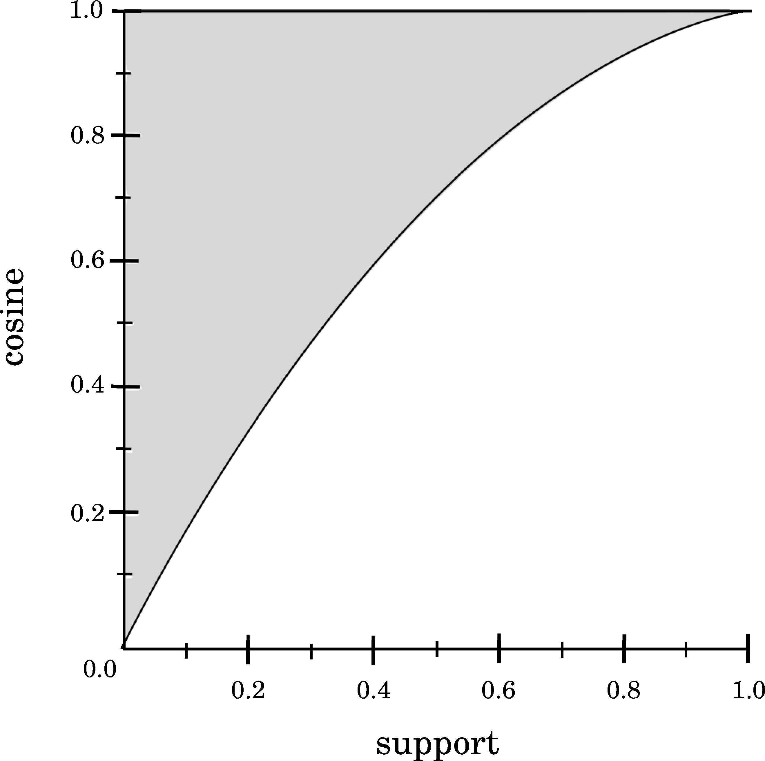
Relationship between Support and Cosine.
On the contrary, minimum Cosine values are obtained when pxy = px (or pxy = py) and py = 1 (or px = 1). Both Support and Cosine behave almost equal to Support and Confidence. In this sense, it is not possible to obtain a high Support value and a low Cosine value at the same time (see Figure 4). This analysis reveals that high Support values imply high Cosine values, but the opposite is not true. Finally, comparing Cosine with Confidence (the feasible area is shown in Figure 5), it is obtained that almost any Confidence value may produce any Cosine value. Hence, both measures can be minimized/maximized at once.
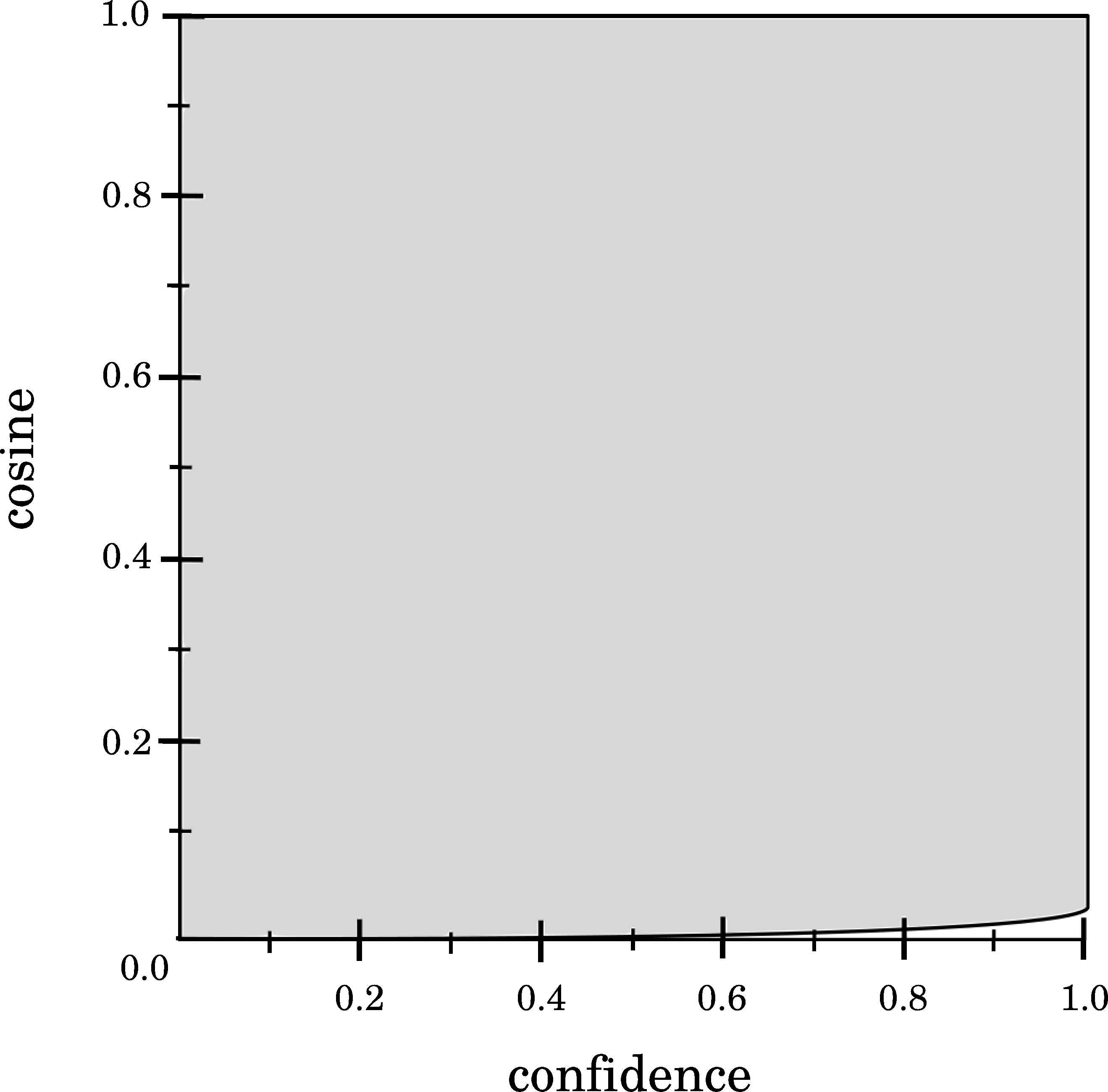
Relationship between Confidence and Cosine.
Leverage vs Support/Confidence.
Leverage, defined as Leverage(X → Y) = pxy − (px × py), determines how different is the co-occurrence of the antecedent X and the consequent Y of a rule from independence10. Similarly to the previous analyses, Figure 6 graphically shows how Support and Leverage are related, denoting that any association rule will obtain a Leverage value in the range [−0.25,0.25] and high Support values tend to produce Leverage values close to 0. The upper boundary of the feasible area is obtained when pxy = px = py, so considering Support(X → Y) = pxy the upper boundary is defined as Leverage(X → Y) = Support(X → Y) − Support2(X → Y). Continuing the analysis, it is obtained that low Support values tend to produce Leverage values lower than 0.
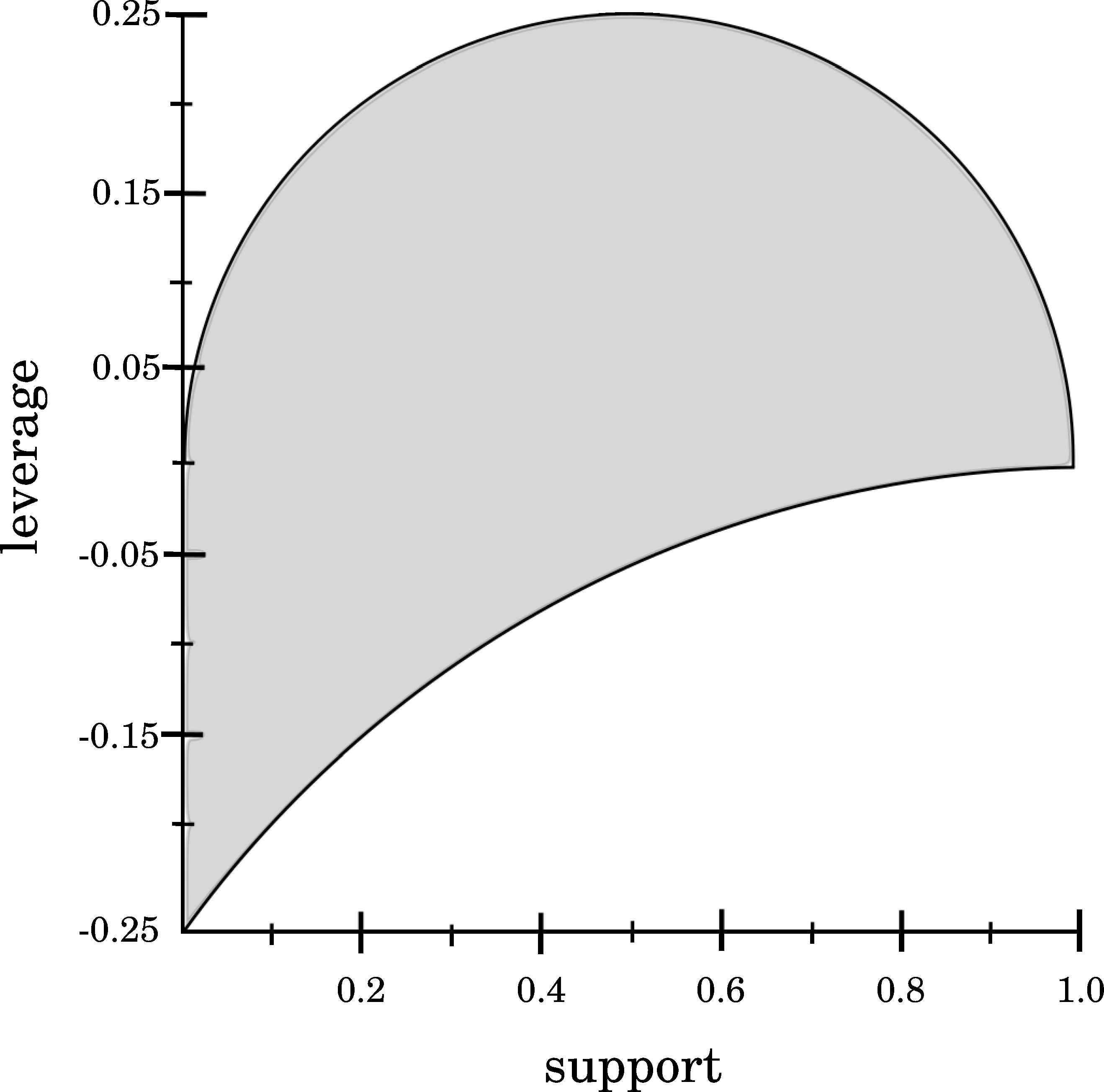
Relationship between Support and Leverage.
Finally, considering how Confidence is related to Leverage (see Figure 7), it is shown that high Confidence values tend to produce positive values for the Leverage quality measure. On the other hand, low Confidence values tend to produce negative values for Leverage. It is interesting to know beforehand that extremely high Confidence values cannot produce negative Leverage values, whereas extremely low Confidence values cannot produce positive Leverage values.
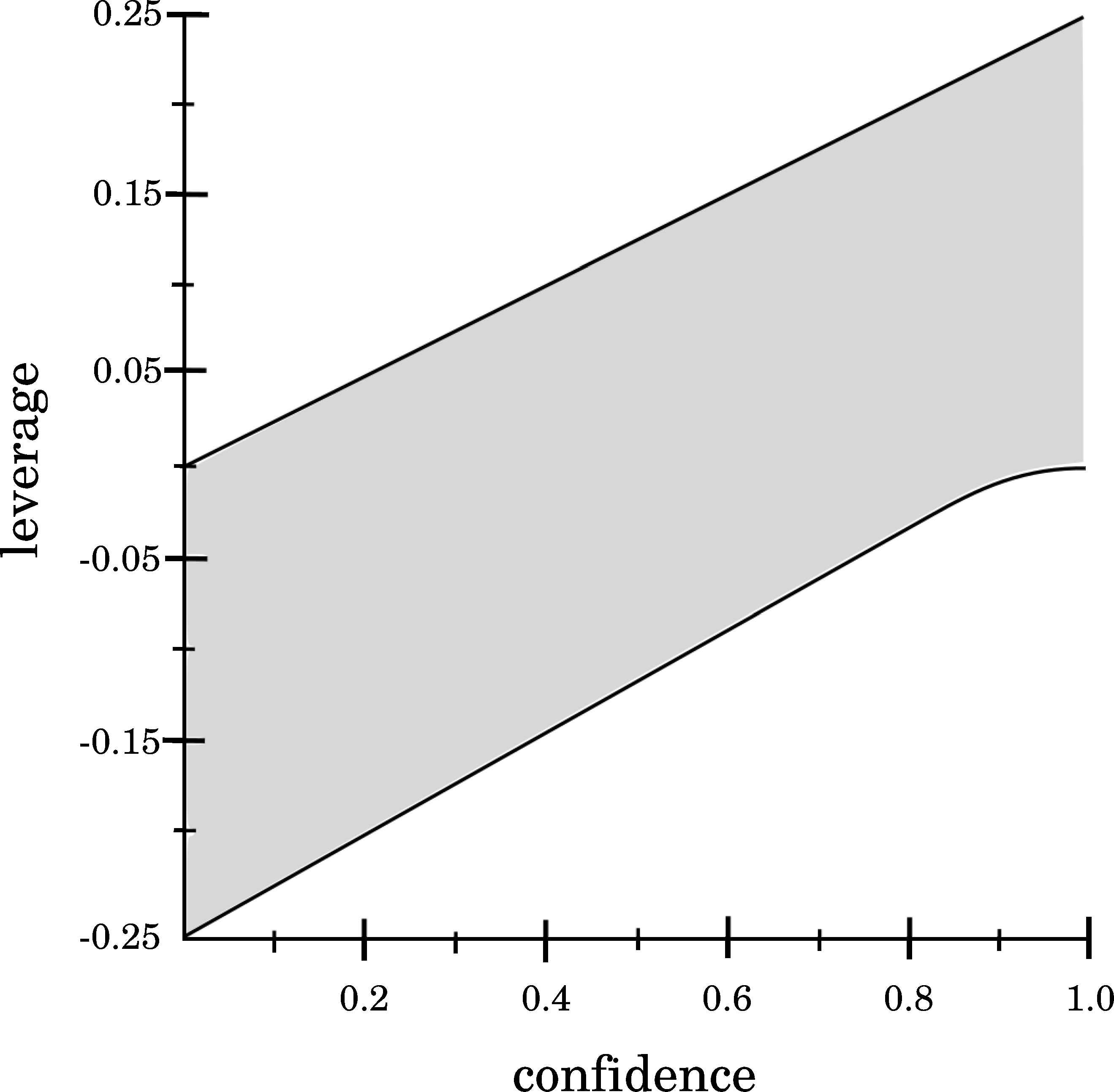
Relationship between Confidence and Leverage.
Conviction vs Support/Confidence.
As shown in Figure 8, Support and Conviction are related in such a way that the highest Conviction values are obtained for intermediate values of Support. Zero Support values (pxy = 0) imply Conviction values defined as Conviction(X → Y)=(px − (px × py))/px=1 − py. Hence, pxy = 0 implies a Conviction value in the range [0,1]. For py = 1 then Conviction(X → Y) = 0, whereas for py = 0 then Conviction(X → Y) = 1. On the contrary, maximum Support values, i.e. pxy = 1, produces invalid Conviction results, since pxy = px = py = 1 and Conviction(X → Y) = 0/0. Hence, it is required to know that no algorithm is able to obtain rules with huge Support values and huge Conviction values regardless the dataset used or the application field.
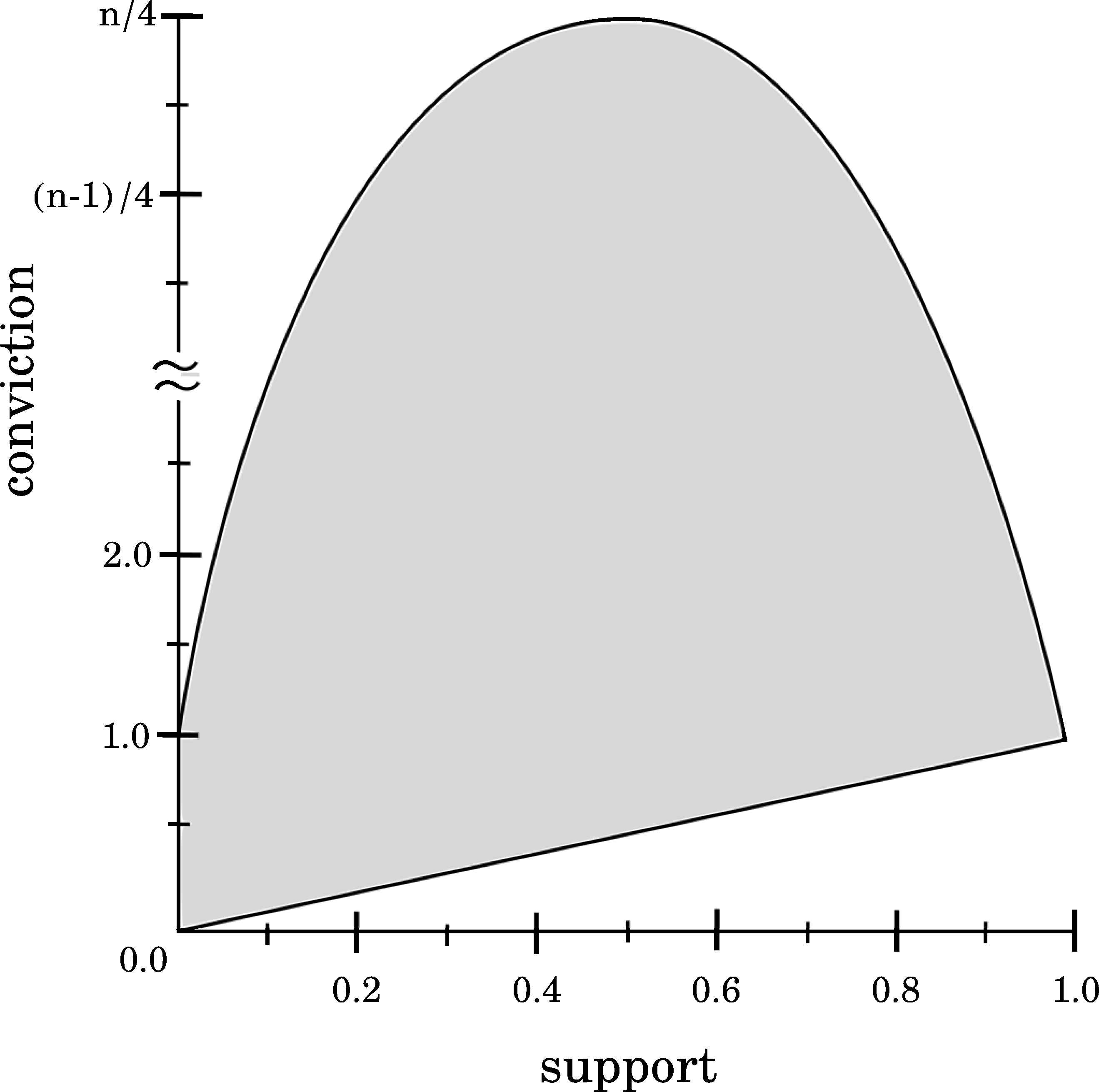
Relationship between Support and Conviction.
Considering now the relationship between Confidence and Conviction (see Figure 9), maximum Confidence values (pxy/px = 1) produce invalid results since pxy = px so Conviction(X → Y) = (1 − pxy)/0. Finally, it should be noted that minimum Confidence values (pxy/px = 0, pxy = 0 and px ≠ 1) implies a Conviction value in the range [0,1]. From this analysis, it is revealed that no association rule can produce a low Confidence value and a high Conviction value at time.
Relationship between Confidence and Conviction.
3. Experimental study
The aim of this experimental study is to analyse a wide set of quality measures in the field of association rule mining, providing the reader with a general knowledge of their behaviour to ease the process of selecting one or more measures when tackling an association rule mining problem. This empirical analysis is a strong point of this paper, including twenty metrics, thirty datasets, and a diverse set of evolutionary algorithms that optimize a single measure12,13,15,20,25 or multiple metrics at time6,27). Here, the ultimate goal is to provide an extensive analysis about how existing quality measures in the association rule mining field are related from different points of view, describing the effects of choosing different metrics as functions to be optimized by any evolutionary algorithm, that is, how values of other measures increase when the values of specific measure are maximized.
The experimental study is performed as follows. First, the collection of datasets used to carry out the experimental analysis is described. Then, the methodology used to achieve an optimization on different quality measures is explained in depth. Finally, the analysis of the quality measures by considering either single-objective and multi-objective optimization methods is performed.
3.1. Datasets
The experimental analysis has been carried out by considering a set of 30 varied and well-known datasets (see Table 3), which are publicly available at http://keel.es, as well as twenty quality measures widely used in the association rule mining field. Datasets were selected to be as varied as possible, including either continuous and discrete attributes, and comprising a diverse number of transactions. This diversity is a keystone since each quality measure may differently behave from dataset to dataset, so the higher the number of datasets, the more close to the reality are the results.
| Dataset | #Attributes | #Discrete | #Continuous | #Transactions |
|---|---|---|---|---|
| AnkaraWeather | 10 | 0 | 10 | 1,609 |
| Automobile | 8 | 0 | 8 | 392 |
| Bolts | 8 | 0 | 8 | 40 |
| Car | 6 | 6 | 0 | 1,728 |
| Chess | 36 | 36 | 0 | 3,196 |
| Cmc | 10 | 3 | 7 | 1,730 |
| Flare | 12 | 12 | 0 | 1,066 |
| German | 20 | 13 | 7 | 1,000 |
| IzmirWeather | 10 | 0 | 10 | 1,461 |
| Marketing | 13 | 13 | 0 | 8,993 |
| Mushrooms | 22 | 22 | 0 | 8,124 |
| Nursery | 8 | 8 | 0 | 12,960 |
| Optdigits | 64 | 0 | 64 | 5,620 |
| Pollution | 16 | 0 | 16 | 60 |
| Ring | 20 | 0 | 20 | 7,400 |
| Satimage | 36 | 0 | 36 | 6,435 |
| Soybean | 36 | 36 | 0 | 683 |
| Stock | 10 | 0 | 10 | 950 |
| Stulong | 5 | 0 | 5 | 1,417 |
| Texture | 40 | 0 | 40 | 5,500 |
| Thyroid | 21 | 0 | 21 | 7,200 |
| Tic-tac-toe | 9 | 9 | 0 | 958 |
| Treasury | 16 | 0 | 16 | 1,049 |
| Twonorm | 20 | 0 | 20 | 7,400 |
| Vote | 16 | 16 | 0 | 435 |
| Vowel | 14 | 4 | 10 | 990 |
| WDatabaseBC | 11 | 1 | 10 | 683 |
| Weather | 5 | 5 | 0 | 14 |
| WPBC | 34 | 1 | 33 | 194 |
| Zoo | 17 | 16 | 1 | 101 |
Datasets (alphabetically ordered) used in the experimental study.
As shown in Table 3, the selected datasets comprise a number of attributes that varies from 5 to 64, whereas the number of transactions ranges from 14 to 12,960. Additionally, the datasets considered in this experimental analysis comprise either discrete and continuous attributes, and the proportion of discrete/continuous attributes varies from dataset to dataset.
3.2. Methodology
The huge number of existing objective quality measures prompts users to carry out an arduous process of choosing the most suitable metrics to be maximized by any algorithm, either exhaustive search or evolutionary methods. In order to get an idea of the role played by each quality measure in this optimization process, a deep analysis is required to determine how each measure behaves when others are optimized. In this regard, the experimental study requires to know beforehand the maximum feasible value for each dataset and quality measure. The previous knowledge of these maximum values eases the process of testing whether a specific quality measure is being optimized or not. It is noteworthy that the maximum value may be completely different from dataset to dataset depending on the data distribution and, therefore, sub-ranges of the ranges analysed in Table 1 should be considered.
Table 4 contains the maximum values for each dataset and quality measure, and it will serve as baseline for the experimental study performed in this work. Any value shown in Table 4 was obtained after running different association rule mining algorithms on each dataset, and keeping the maximum value obtained for each quality measure. In those datasets that only include discrete attributes, then a brute force algorithm9 was applied, which extracts any existing association rule, so the maximum value for each dataset can be surely obtained. However, this kind of algorithms cannot be applied to datasets comprising continuous attributes due to the huge search space. For these specific datasets, the extraction of the maximum value for each quality measure is not a trivial issue since each continuous attribute can be split into an undetermined number of bins. Hence, the same brute force algorithm9 was applied by transforming continuous attributes into a varied number of bins (equal-width and equal-frequency binning methods were applied, considering 5, 10, 15, 20, 25 and 30 bins). Additionally, different evolutionary algorithms (NICGAR15, EARMGA-A25, ARMMGA20, QuantG3P12 and G3PARM13) that work with continuous attributes without a previous transformation were also considered. These algorithms, which were taken from KEEL23 software tool, were specifically designed to work with continuous attributes and they have achieved a really good performance24. As a result, the values shown in Table 4 are the maximum values obtained after applying all the aforementioned algorithms.
| Dataset | Support | Coverage | Prevalence | Confidence | Lift | Cosine | Leverage | Conviction | CC | CF | Recall | Laplace | Pearson | IG | Sebag | LC | ECR | Zhang | Netconf | Yule’sQ |
|---|---|---|---|---|---|---|---|---|---|---|---|---|---|---|---|---|---|---|---|---|
| AnkaraWeather | 1.00 | 1.00 | 1.00 | 1.00 | 1,609.00 | 1.00 | 0.23 | 302.70 | 1.00 | 1.00 | 1.00 | 1.00 | 1.00 | 7.38 | 1,597.80 | 1.00 | 1.00 | 1.00 | 1.00 | 1.00 |
| Automobile | 1.00 | 1.00 | 1.00 | 1.00 | 392.00 | 1.00 | 0.24 | 91.60 | 1.00 | 1.00 | 1.00 | 1.00 | 0.98 | 5.97 | 377.20 | 1.00 | 1.00 | 1.00 | 1.00 | 1.00 |
| Bolts | 1.00 | 1.00 | 1.00 | 1.00 | 40.00 | 1.00 | 0.18 | 7.80 | 0.98 | 1.00 | 1.00 | 0.98 | 1.00 | 3.69 | 0.00 | 1.00 | 1.00 | 1.00 | 1.00 | 1.00 |
| Car | 0.11 | 0.33 | 0.33 | 0.33 | 1.00 | 0.33 | 0.00 | 1.00 | 0.00 | 0.00 | 0.33 | 0.34 | 0.00 | 0.00 | 0.50 | −0.02 | −1.00 | 0.00 | 0.00 | 0.35 |
| Chess | 1.00 | 1.00 | 1.00 | 1.00 | 2,876.40 | 1.00 | 0.18 | 429.50 | 1.00 | 1.00 | 1.00 | 1.00 | 0.96 | 7.93 | 3,184.30 | 1.00 | 1.00 | 1.00 | 1.00 | 1.00 |
| Cmc | 1.00 | 1.00 | 1.00 | 1.00 | 1,473.00 | 1.00 | 0.14 | 60.80 | 1.00 | 1.00 | 1.00 | 1.00 | 0.65 | 7.30 | 1,472.00 | 1.00 | 1.00 | 1.00 | 1.00 | 1.00 |
| Flare | 0.97 | 1.00 | 1.00 | 1.00 | 1,066.00 | 1.00 | 0.21 | 157.60 | 1.00 | 1.00 | 1.00 | 1.00 | 1.00 | 6.97 | 1,038.00 | 1.00 | 1.00 | 1.00 | 1.00 | 0.99 |
| German | 1.00 | 1.00 | 1.00 | 1.00 | 1,000.00 | 1.00 | 0.14 | 61.50 | 1.00 | 1.00 | 1.00 | 1.00 | 1.00 | 6.91 | 896.20 | 1.00 | 1.00 | 1.00 | 1.00 | 1.00 |
| IzmirWeather | 1.00 | 1.00 | 1.00 | 1.00 | 1,461.00 | 1.00 | 0.23 | 300.90 | 1.00 | 1.00 | 1.00 | 1.00 | 0.97 | 7.29 | 1,457.90 | 1.00 | 1.00 | 1.00 | 1.00 | 1.00 |
| Marketing | 1.00 | 1.00 | 1.00 | 1.00 | 6,876.00 | 1.00 | 0.22 | 423.30 | 1.00 | 1.00 | 1.00 | 1.00 | 0.95 | 8.84 | 0.00 | 1.00 | 1.00 | 1.00 | 1.00 | 1.00 |
| Mushrooms | 0.98 | 1.00 | 1.00 | 1.00 | 1,015.50 | 1.00 | 0.21 | 172.10 | 1.00 | 1.00 | 1.00 | 1.00 | 1.00 | 6.92 | 1,547.90 | 1.00 | 1.00 | 1.00 | 1.00 | 1.00 |
| Nursery | 0.33 | 0.50 | 0.50 | 1.00 | 240.00 | 1.00 | 0.22 | 66.00 | 1.00 | 1.00 | 1.00 | 1.00 | 1.00 | 5.48 | 0.00 | 1.00 | 1.00 | 1.00 | 1.00 | 0.50 |
| Optdigits | 1.00 | 1.00 | 1.00 | 1.00 | 4,215.00 | 1.00 | 0.13 | 82.70 | 1.00 | 1.00 | 1.00 | 1.00 | 0.94 | 8.22 | 0.00 | 1.00 | 1.00 | 1.00 | 1.00 | 1.00 |
| Pollution | 0.95 | 0.97 | 0.97 | 1.00 | 60.00 | 1.00 | 0.19 | 10.40 | 0.98 | 1.00 | 1.00 | 0.98 | 1.00 | 4.09 | 57.00 | 1.00 | 1.00 | 1.00 | 1.00 | 0.94 |
| Ring | 1.00 | 1.00 | 1.00 | 1.00 | 7,400.00 | 1.00 | 0.10 | 15.30 | 1.00 | 1.00 | 1.00 | 1.00 | 0.50 | 8.91 | 0.00 | 1.00 | 1.00 | 1.00 | 1.00 | 1.00 |
| Satimage | 1.00 | 1.00 | 1.00 | 1.00 | 5,577.00 | 1.00 | 0.21 | 705.40 | 1.00 | 1.00 | 1.00 | 1.00 | 0.91 | 8.13 | 0.00 | 1.00 | 1.00 | 1.00 | 1.00 | 1.00 |
| Soybean | 0.91 | 0.94 | 0.94 | 1.00 | 683.00 | 1.00 | 0.24 | 152.40 | 1.00 | 1.00 | 1.00 | 1.00 | 1.00 | 6.25 | 480.40 | 1.00 | 1.00 | 1.00 | 1.00 | 0.89 |
| Stock | 0.99 | 1.00 | 1.00 | 1.00 | 950.00 | 1.00 | 0.24 | 194.20 | 1.00 | 1.00 | 1.00 | 1.00 | 0.98 | 6.86 | 911.60 | 0.99 | 1.00 | 1.00 | 1.00 | 0.99 |
| Stulong | 1.00 | 1.00 | 1.00 | 1.00 | 1,417.00 | 1.00 | 0.14 | 73.70 | 1.00 | 1.00 | 1.00 | 1.00 | 1.00 | 7.26 | 1,415.20 | 1.00 | 1.00 | 1.00 | 1.00 | 1.00 |
| Texture | 1.00 | 1.00 | 1.00 | 1.00 | 5,500.00 | 1.00 | 0.23 | 825.90 | 1.00 | 1.00 | 1.00 | 1.00 | 1.00 | 8.61 | 0.00 | 1.00 | 1.00 | 1.00 | 1.00 | 1.00 |
| Thyroid | 1.00 | 1.00 | 1.00 | 1.00 | 7,200.00 | 1.00 | 0.14 | 46.70 | 1.00 | 1.00 | 1.00 | 1.00 | 1.00 | 8.88 | 0.00 | 1.00 | 1.00 | 1.00 | 1.00 | 1.00 |
| Tic-tac-toe | 0.38 | 0.65 | 0.65 | 1.00 | 958.00 | 0.68 | 0.08 | 13.50 | 0.99 | 1.00 | 1.00 | 0.99 | 0.48 | 6.86 | 0.00 | 0.44 | 1.00 | 1.00 | 0.99 | 0.59 |
| Treasury | 0.99 | 0.99 | 0.99 | 1.00 | 1,049.00 | 1.00 | 0.24 | 225.50 | 1.00 | 1.00 | 1.00 | 1.00 | 0.98 | 6.96 | 967.80 | 0.99 | 1.00 | 1.00 | 1.00 | 0.99 |
| Twonorm | 1.00 | 1.00 | 1.00 | 1.00 | 7,400.00 | 1.00 | 0.06 | 15.90 | 1.00 | 1.00 | 1.00 | 1.00 | 0.88 | 8.91 | 0.00 | 1.00 | 1.00 | 1.00 | 1.00 | 1.00 |
| Vote | 0.56 | 0.63 | 0.63 | 1.00 | 435.00 | 0.96 | 0.22 | 93.10 | 1.00 | 1.00 | 1.00 | 1.00 | 0.91 | 6.08 | 210.00 | 0.95 | 1.00 | 1.00 | 1.00 | 0.60 |
| Vowel | 1.00 | 1.00 | 1.00 | 1.00 | 990.00 | 1.00 | 0.14 | 55.10 | 1.00 | 1.00 | 1.00 | 1.00 | 0.90 | 6.76 | 987.80 | 1.00 | 1.00 | 1.00 | 1.00 | 1.00 |
| WDatabaseBC | 1.00 | 1.00 | 1.00 | 1.00 | 683.00 | 1.00 | 0.20 | 102.60 | 1.00 | 1.00 | 1.00 | 1.00 | 0.87 | 6.53 | 579.00 | 1.00 | 1.00 | 1.00 | 1.00 | 1.00 |
| Weather | 0.43 | 0.64 | 0.64 | 1.00 | 7.00 | 1.00 | 0.14 | 2.60 | 0.86 | 1.00 | 1.00 | 0.83 | 1.00 | 1.95 | 6.00 | 1.00 | 1.00 | 1.00 | 1.00 | 0.61 |
| WPBC | 0.99 | 0.99 | 1.00 | 1.00 | 194.00 | 1.00 | 0.24 | 41.40 | 0.99 | 1.00 | 1.00 | 0.99 | 1.00 | 5.27 | 190.60 | 1.00 | 1.00 | 1.00 | 1.00 | 0.99 |
| Zoo | 0.92 | 1.00 | 1.00 | 1.00 | 101.00 | 1.00 | 0.24 | 24.80 | 0.99 | 1.00 | 1.00 | 0.99 | 1.00 | 4.62 | 74.00 | 1.00 | 1.00 | 1.00 | 1.00 | 1.00 |
Maximum feasible values found for each dataset and each quality measure.
The methodology followed in this work is based on checking whether each quality measure is being optimized or not. We determine that a specific quality measure is being optimized if the results for this measure is close to the maximum value described in Table 4. For instance, let us consider the ankara weather dataset and a sample rule having the values for Support and Confidence equal to 0.90 and 0.92, respectively. In such a situation, it is possible to assert that both quality measures are optimized at time since the maximum values for both Support and Confidence measures are 1.00. Let us also consider now a sample rule on dataset nursery having the values for Support and Confidence equal to 0.32 and 0.98, respectively. In this situation, it is also possible to assert that the rule optimizes both quality measures at time since the maximum Support value is 0.33, and 1.00 for the Confidence metric for this specific dataset. Therefore, it demonstrates that the optimization testing should be carried out by considering the maximum values for each specific dataset and not only the maximum feasible values mathematically described in Table 2.
The empirical analysis is twofold: single and multiple objective optimization. As for single-objective optimization, the aim is to determine a single measure as objective to be optimized, and to test how the rest of measures behave. The process is repeated by each single quality measure. An exhaustive search algorithm9 and a set of evolutionary algorithms (NICGAR15, EARMGA-A25, ARMMGA20, QuantG3P12 and G3PARM13) freely available in the KEEL23 software tool was performed, and each algorithm was run 6,000 times — evolutionary algorithms are stochastic models so 10 different runs per dataset and per quality measure are required. Results are the average results obtained for the different runs and taking the top rules discovered, i.e. those having the highest value for the objective quality measure. We have taken a resulting set of 20 rules since this is the number most widely used by most of the evolutionary algorithms for discovering the top association rules24. As for multi-objective optimization, two of the most well-known multi-objective optimization algorithms were used (NSGA26 and SPEA227), and each one was run 57,000 times — they are stochastic algorithms so 10 different runs per dataset and per pair of quality measures (190 combinations of quality measures). Results are the average results obtained for the different runs and taking the resulting set of rules (the ones that achieve a good trade-off between two conflicting metrics) of each algorithm.
3.3. Single-objective optimization
In this first analysis, a single-objective optimization is performed by taking each sole quality measure as objective function each time. The aim is three-fold: first, to check which quality measure is maximized by a higher number of other quality measures; second, to determine which quality measure (used as a single objective function) allows a higher number of quality measures to be optimized (maximized) at time; finally, to analyse which set of quality measures should be used to maximize all the metrics. A specific quality measure is marked as optimized if it is close to the maximum value according to a specific percentile. As a matter of example, the Support quality measure whose values range in the interval [0.0,1.0] will be marked as optimized in the 90th percentile if a value is in the range [0.9,1.0].
First analysis.
Taking the aforementioned guidelines, the first goal is to check which quality measures is optimized by a higher number of objectives (single quality measures). As previously demonstrated, the percentile used to mark whether a quality measure has been optimized or not plays a really important role since minimum/maximum values changed from dataset to dataset. Hence, for the sake of doing a complete analysis, different percentiles (70th, 80th and 90th percentile) were considered. Results are summarized in Figure 10, which shows the percentage of objective functions that optimize each single quality. As it is illustrated, Confidence and ECR are optimized by almost 80% of the objective functions. Additionally, Zhang and CF (Certainty Factor) are also really general quality measures, since they are optimized by close to 70% of the objectives (single metrics). On the contrary, Support, Lift, Leverage, Conviction, IG, Sebag and Yule’sQ are high indepedent quality measures since they are hardly optimized by any other single metric.
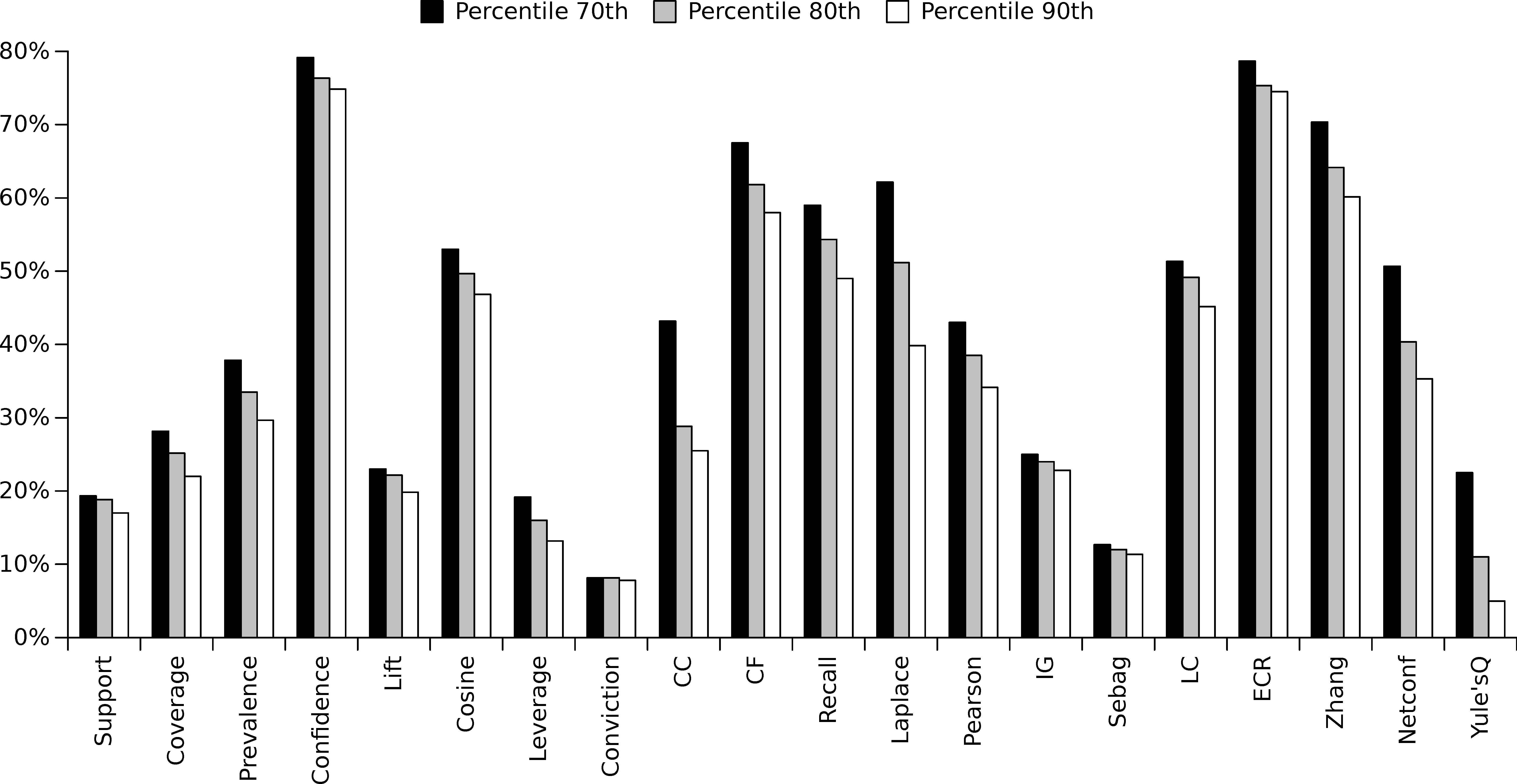
Percentage of objective functions that optimize each quality measure by considering different percentiles (70th, 80th and 90th percentile).
Taking those quality measures (Confidence, CF, Laplace, ECR and Zhang) that are optimized by a higher number of fitness functions (single quality measures) according to the previous analysis summarized in Figure 10, the aim is to check the behaviour on each single dataset. In this sense, Table 5 shows the results for this analysis, stating that Confidence and ECR are optimized by around 80% of the quality measures regardless the dataset used and with a low dispersion. As for the Confidence quality measure, it is optimized by more than 70% of the quality measures for any dataset except for Treasury and Weather. The latter is, according to the results, the dataset in which the Confidence quality measure worst behaves since this measure is maximized by only 40% of the metrics.
| Dataset | Confidence | CF | Laplace | ECR | Zhang |
|---|---|---|---|---|---|
| Ankara weather | 0.85 | 0.55 | 0.65 | 0.85 | 0.55 |
| Automobile | 0.85 | 0.75 | 0.65 | 0.85 | 0.75 |
| Bolts | 0.85 | 0.70 | 0.75 | 0.85 | 0.70 |
| Car | 0.85 | 0.50 | 0.65 | 0.75 | 0.50 |
| Chess | 0.85 | 0.50 | 0.60 | 0.85 | 0.55 |
| Cmc | 0.80 | 0.70 | 0.65 | 0.80 | 0.70 |
| Flare | 0.70 | 0.65 | 0.75 | 0.70 | 0.70 |
| German | 0.75 | 0.80 | 0.75 | 0.75 | 0.90 |
| Izmir weather | 0.85 | 0.85 | 0.70 | 0.85 | 0.85 |
| Marketing | 0.80 | 0.80 | 0.65 | 0.80 | 0.85 |
| Mushrooms | 0.80 | 0.60 | 0.60 | 0.80 | 0.65 |
| Nursery | 0.80 | 0.70 | 0.50 | 0.80 | 0.70 |
| Optdigits | 0.85 | 0.70 | 0.70 | 0.85 | 0.70 |
| Pollution | 0.80 | 0.60 | 0.70 | 0.75 | 0.60 |
| Ring | 0.80 | 0.75 | 0.65 | 0.80 | 0.75 |
| Satimage | 0.70 | 0.75 | 0.70 | 0.65 | 0.85 |
| Soybean | 0.80 | 0.80 | 0.50 | 0.80 | 0.85 |
| Stock | 0.80 | 0.80 | 0.60 | 0.80 | 0.80 |
| Stulong | 0.80 | 0.65 | 0.50 | 0.75 | 0.65 |
| Texture | 0.85 | 0.70 | 0.65 | 0.80 | 0.70 |
| Thyroid | 0.85 | 0.75 | 0.60 | 0.75 | 0.75 |
| Tic-tac-toe | 0.80 | 0.75 | 0.65 | 0.80 | 0.75 |
| Treasury | 0.65 | 0.65 | 0.40 | 0.60 | 0.85 |
| Twonorm | 0.80 | 0.50 | 0.65 | 0.70 | 0.50 |
| Vote | 0.85 | 0.40 | 0.65 | 0.80 | 0.40 |
| Vowel | 0.80 | 0.85 | 0.60 | 0.80 | 0.90 |
| WDatabaseBC | 0.85 | 0.40 | 0.70 | 0.85 | 0.45 |
| Weather | 0.40 | 0.85 | 0.40 | 0.90 | 0.85 |
| WPBC | 0.80 | 0.60 | 0.60 | 0.75 | 0.60 |
| Zoo | 0.80 | 0.65 | 0.50 | 0.80 | 0.75 |
Average percentage (in per unit basis) of objective functions that achieves to optimize the measures analysed for each dataset. The 70th percentile was considered.
Focusing now on the ECR quality measure, it is optimized by more than 70% of the quality measures for any dataset except for Satimage and Treasury. This is a normal behaviour since data distribution from dataset to dataset may vary so much. Thus, it is important to analyse the results from a general perspective, taking as many datasets as possible. Finally, it is noteworthy that the analysis performed provides the user with a really interesting knowledge, denoting that Confidence and ECR may be optimized without fixing them implicitly into the function to be optimized. At the same time, other quality measures such as Lift or Leverage cannot be optimized unless they are included into the function to be optimized (see Figure 10).
Second analysis.
The next analysis of this experimental stage is to determine those single-objectives that enable a higher number of different metrics to be maximized. In this regard, and similarly to the previous analysis, three different percentiles (70th, 80th and 90th percentile) has been considered. The results obtained for all the datasets under study have been summarized in Figure 11, which shows the percentage of measures that are maximized by each single-objective. As it is illustrated, Coverage, Prevalence, Recall and Yule’sQ optimize an extremely low number of quality measures. Hence, it is possible to assert that these metrics should be avoided as single-objective functions in those situations were values close to the maximum are required in other quality measures. Continuing the analysis, there is no specific objective function that enables a high number of metrics to be optimized. As shown in Figure 11, the optimization of any single measure produces a maximization in less than 60% of the metrics. From all the analysed single-objective functions, Lift, CC, Pearson, IG and Netconf are the most promising ones, achieving to optimize more than 50% of the quality measures at time.
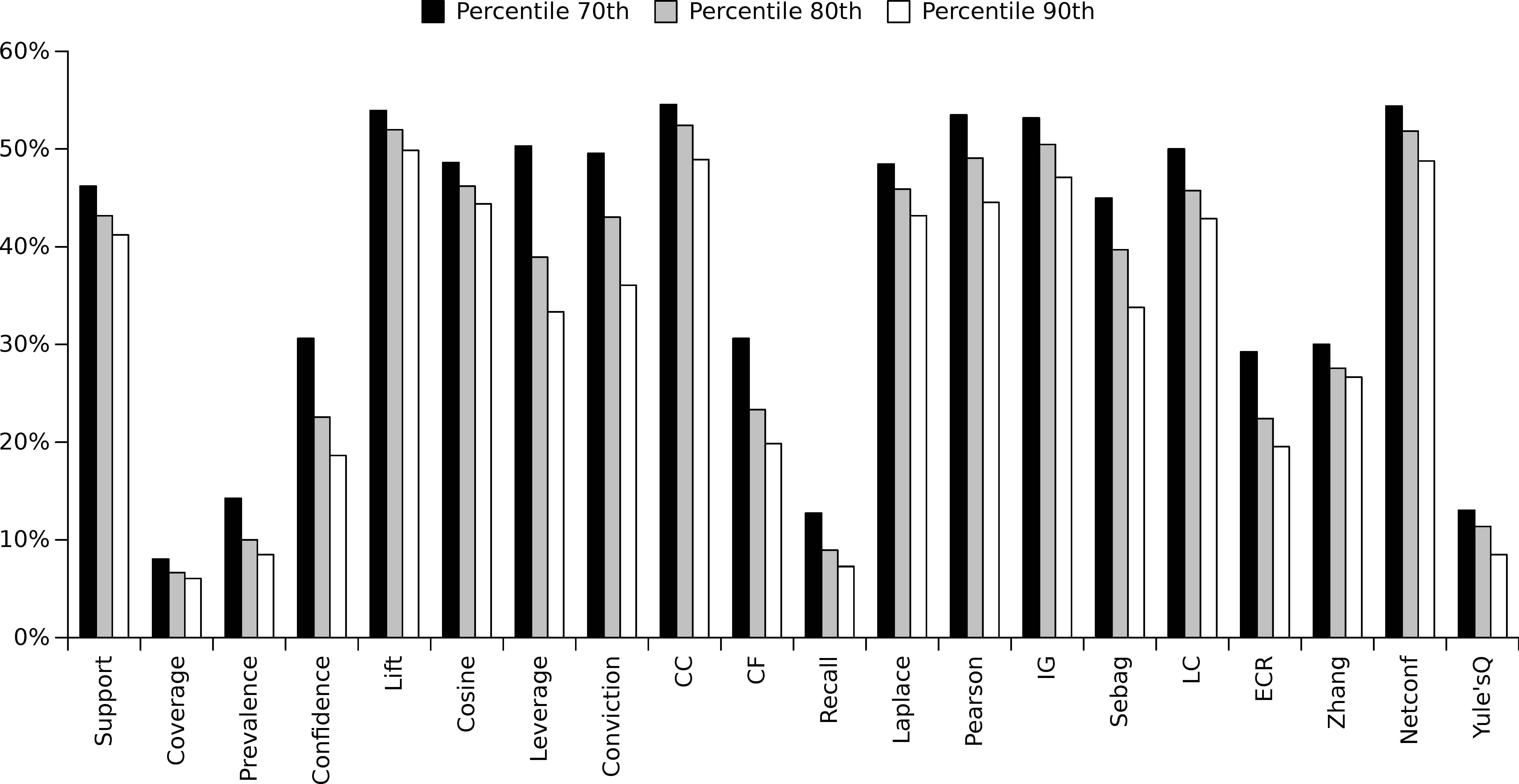
Average percentage of quality measures that were optimized by each single-objective and considering different percentiles (70th, 80th and 90th percentile).
Third analysis.
The last analysis is conducted to determine which set of quality measures should be used to maximize the whole set of quality measures. Let us consider Support as the best known quality measure in the association rule mining field and, at the same time, it was defined as the quality measure that maximizes a higher number of quality measures at time. Hence, this metric will be taken as baseline. Analysing the results shown in Table 6, it is obtained that Support enables the following metrics to be maximized (taking those satisfied in >90% of the datasets): Support, Coverage, Prevalence, Confidence, Cosine, Recall, Laplace, Least Contradiction (LC) and ECR. Hence, none of these metrics should be taken if Support was previously used as an objective function to be maximized. Continuing the analysis, and discarding from Table 6 those quality measure already maximized by Support (these columns are obtained by now), it is obtained that Lift maximizes the following (taking those satisfied in >90% of the datasets): Lift, CC, CF, Pearson, IG, Zhang and Netconf. The rest of the quality measures, i.e. those that has not been maximized yet neither by Support nor by Lift, are only maximized by themselves. Thus, Leverage, Conviction, Sebag and Yule’sQ are also required as quality measures to be optimized.
| Objective function | Support | Coverage | Prevalence | Confidence | Lift | Cosine | Leverage | Conviction | CC | CF | Recall | Laplace | Pearson | IG | Sebag | LC | ECR | Zhang | Netconf | Yule’sQ |
|---|---|---|---|---|---|---|---|---|---|---|---|---|---|---|---|---|---|---|---|---|
| Support | 1.00 | 0.97 | 0.97 | 0.97 | 0.00 | 1.00 | 0.13 | 0.00 | 0.03 | 0.20 | 1.00 | 0.97 | 0.20 | 0.00 | 0.33 | 0.97 | 0.93 | 0.27 | 0.17 | 0.07 |
| Coverage | 0.00 | 1.00 | 0.00 | 0.00 | 0.03 | 0.00 | 0.03 | 0.03 | 0.03 | 0.03 | 0.27 | 0.00 | 0.03 | 0.03 | 0.10 | 0.00 | 0.00 | 0.03 | 0.03 | 0.10 |
| Prevalence | 0.00 | 0.00 | 1.00 | 0.40 | 0.00 | 0.03 | 0.03 | 0.00 | 0.00 | 0.17 | 0.00 | 0.57 | 0.03 | 0.00 | 0.17 | 0.03 | 0.40 | 0.17 | 0.00 | 0.13 |
| Confidence | 0.00 | 0.00 | 0.50 | 1.00 | 0.03 | 0.03 | 0.07 | 0.03 | 0.37 | 0.93 | 0.00 | 1.00 | 0.03 | 0.03 | 0.03 | 0.03 | 1.00 | 0.93 | 0.43 | 0.27 |
| Lift | 0.00 | 0.00 | 0.00 | 0.90 | 1.00 | 0.90 | 0.07 | 0.03 | 1.00 | 1.00 | 0.90 | 0.03 | 0.97 | 1.00 | 0.00 | 0.87 | 0.90 | 1.00 | 1.00 | 0.30 |
| Cosine | 0.60 | 0.57 | 0.57 | 0.97 | 0.17 | 1.00 | 0.23 | 0.00 | 0.40 | 0.47 | 1.00 | 0.83 | 0.50 | 0.20 | 0.17 | 1.00 | 0.97 | 0.50 | 0.47 | 0.10 |
| Leverage | 0.03 | 0.00 | 0.00 | 0.90 | 0.03 | 0.93 | 1.00 | 0.07 | 0.63 | 0.93 | 0.90 | 0.90 | 0.97 | 0.03 | 0.30 | 0.67 | 0.73 | 1.00 | 0.93 | 0.10 |
| Conviction | 0.00 | 0.00 | 0.17 | 0.93 | 0.03 | 0.57 | 0.63 | 1.00 | 0.73 | 1.00 | 0.43 | 0.93 | 0.73 | 0.07 | 0.37 | 0.43 | 0.97 | 1.00 | 0.80 | 0.10 |
| CC | 0.00 | 0.00 | 0.00 | 0.97 | 0.93 | 0.90 | 0.07 | 0.03 | 1.00 | 1.00 | 0.83 | 0.13 | 0.97 | 1.00 | 0.00 | 0.87 | 1.00 | 1.00 | 1.00 | 0.30 |
| CF | 0.00 | 0.00 | 0.37 | 0.97 | 0.03 | 0.00 | 0.07 | 0.03 | 0.40 | 1.00 | 0.00 | 0.97 | 0.03 | 0.03 | 0.00 | 0.03 | 1.00 | 1.00 | 0.47 | 0.33 |
| Recall | 0.00 | 0.63 | 0.00 | 0.00 | 0.03 | 0.00 | 0.10 | 0.03 | 0.07 | 0.07 | 1.00 | 0.00 | 0.10 | 0.03 | 0.03 | 0.03 | 0.03 | 0.37 | 0.07 | 0.20 |
| Laplace | 0.90 | 0.87 | 0.97 | 1.00 | 0.03 | 0.90 | 0.17 | 0.03 | 0.07 | 0.60 | 0.90 | 1.00 | 0.33 | 0.03 | 0.03 | 0.93 | 1.00 | 0.60 | 0.20 | 0.10 |
| Pearson | 0.03 | 0.00 | 0.00 | 0.93 | 0.37 | 0.93 | 0.47 | 0.03 | 1.00 | 1.00 | 0.93 | 0.60 | 1.00 | 0.40 | 0.10 | 0.90 | 0.90 | 1.00 | 1.00 | 0.17 |
| IG | 0.00 | 0.00 | 0.00 | 0.87 | 1.00 | 0.90 | 0.07 | 0.03 | 0.97 | 0.97 | 0.93 | 0.03 | 0.97 | 1.00 | 0.00 | 0.83 | 0.87 | 1.00 | 0.97 | 0.30 |
| Sebag | 0.60 | 0.60 | 0.87 | 1.00 | 0.03 | 0.60 | 0.13 | 0.10 | 0.13 | 0.67 | 0.57 | 1.00 | 0.20 | 0.03 | 0.97 | 0.60 | 1.00 | 0.67 | 0.27 | 0.17 |
| LC | 0.53 | 0.50 | 0.53 | 1.00 | 0.20 | 0.97 | 0.27 | 0.03 | 0.43 | 0.53 | 0.93 | 0.93 | 0.57 | 0.23 | 0.20 | 1.00 | 1.00 | 0.53 | 0.50 | 0.10 |
| ECR | 0.00 | 0.00 | 0.47 | 1.00 | 0.03 | 0.00 | 0.07 | 0.03 | 0.33 | 0.87 | 0.00 | 1.00 | 0.03 | 0.03 | 0.03 | 0.03 | 1.00 | 0.87 | 0.37 | 0.27 |
| Zhang | 0.00 | 0.00 | 0.90 | 0.97 | 0.03 | 0.00 | 0.07 | 0.03 | 0.13 | 1.00 | 0.00 | 0.97 | 0.03 | 0.03 | 0.00 | 0.03 | 1.00 | 1.00 | 0.17 | 0.23 |
| Netconf | 0.17 | 0.13 | 0.13 | 0.97 | 0.57 | 0.93 | 0.13 | 0.03 | 0.87 | 0.87 | 0.93 | 0.57 | 0.87 | 0.77 | 0.00 | 0.97 | 1.00 | 0.90 | 1.00 | 0.17 |
| Yule’sQ | 0.00 | 0.37 | 0.13 | 0.10 | 0.03 | 0.00 | 0.03 | 0.03 | 0.03 | 0.20 | 0.27 | 0.00 | 0.03 | 0.03 | 0.00 | 0.03 | 0.03 | 0.23 | 0.30 | 1.00 |
Average percentage (in per unit basis) of datasets in which each quality measure is maximized when a single measure (objective function) is used as objective to be maximized. The 70th percentile was considered.
3.4. Multi-objective optimization
In this second analysis, a multi-objective optimization is performed by taking any pair of metrics (each quality measure is a different objective) from the set of 20 quality measures analysed in this work. Hence, from a total of 190 existing pairs (number of combinations of pairs of quality measures), the goal is to test which specific group of quality measures is optimized when others are used as multi-objective functions. Similarly to the previous analysis, the final aim is three-fold: first, to check which quality measure is maximized by a higher number of pairs of measures; second, to determine which pair of quality measures (used as multi-objective function) allow a higher number of quality measures to be optimized (maximized) at time; and, finally, to analyse which set of multi-objective functions should be used to maximize all the metrics.
First analysis.
Taking the aforementioned guidelines, the goal of this first analysis is to check which quality measures are optimized by a higher number of objectives (pairs of quality measures). Similarly to the previous experimental study for single-objective optimization, the percentile used to mark a quality measure as optimized is a keystone, so different percentiles (70th, 80th and 90th percentile) were considered to carry out a complete analysis. Figure 12 illustrates the average results obtained for all the runs and considering all the datasets and two well-known multi-objective optimization models (NSGA2 and SPEA2). In this figure, the percentage of objectives (from a total of 190 pairs of quality measures) that optimizes each quality measure by considering different percentiles (70th, 80th and 90th percentile) is shown. As it is illustrated, Coverage, Laplace and zhang are optimized by more than 80% of the 190 pairs of multi-objective functions available in this study. Additionally, CF and ECR are also really general quality measures, since they are optimized by close to 70% of the multi-objectives. On the contrary, Lift, Conviction, IG and Netconf are high independent quality measures since they are hardly optimized by any multi-objective function.
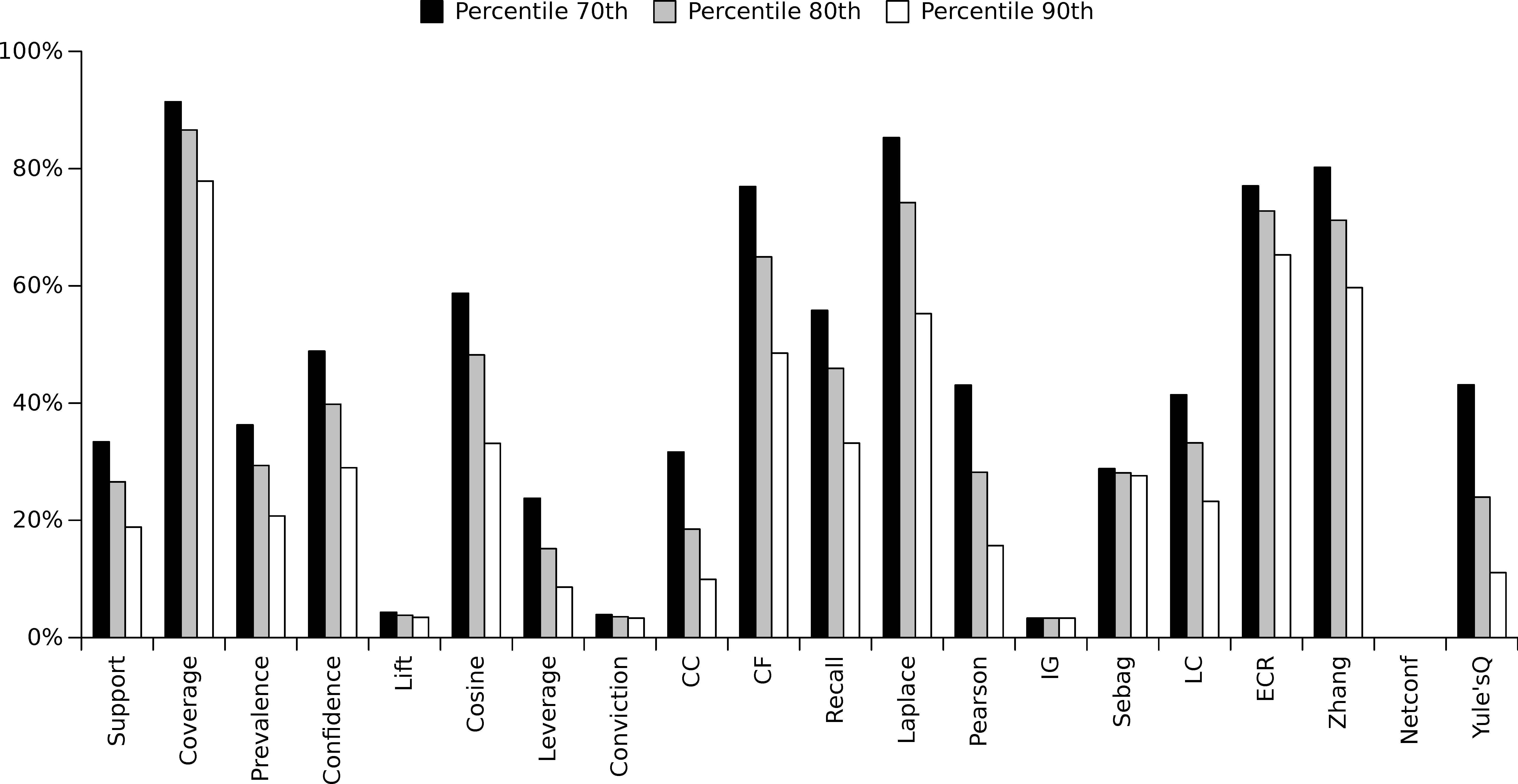
Percentage of pairs of objectives, from a total of 190 pairs, that maximizes each quality measure by considering different percentiles (70th, 80th and 90th percentile).
Second analysis.
The next analysis of this experimental stage is to determine which multi-objectives (pairs of metrics) enable a higher number of metrics to be maximized. In this regard, and similarly to the previous analysis, three different percentiles (70th, 80th and 90th percentile) have been considered. The results obtained for all the datasets under study and considering the 70th percentile have been summarized in Figure 13, which shows the percentage of measures that were maximized by each multi-objective functions (only the 20 multi-objective functions that maximize a higher percentage of quality measures are shown in this analysis). As it is illustrated, there is no specific multi-objective function that enables a high number of metrics to be optimized, and the optimization of any multi-objective function produces a maximization in less than 60% of the metrics. As a remarkable result, it is obtained that more than 56% of the metrics were optimized by the following multi-objective metrics: Support-Leverage, Leverage-LC, CF-LC, and Cosine-Leverage. Finally, the same analysis has been carried out for different percentiles (80th and 90th) and as it is summarized in Figures 14 and 15.
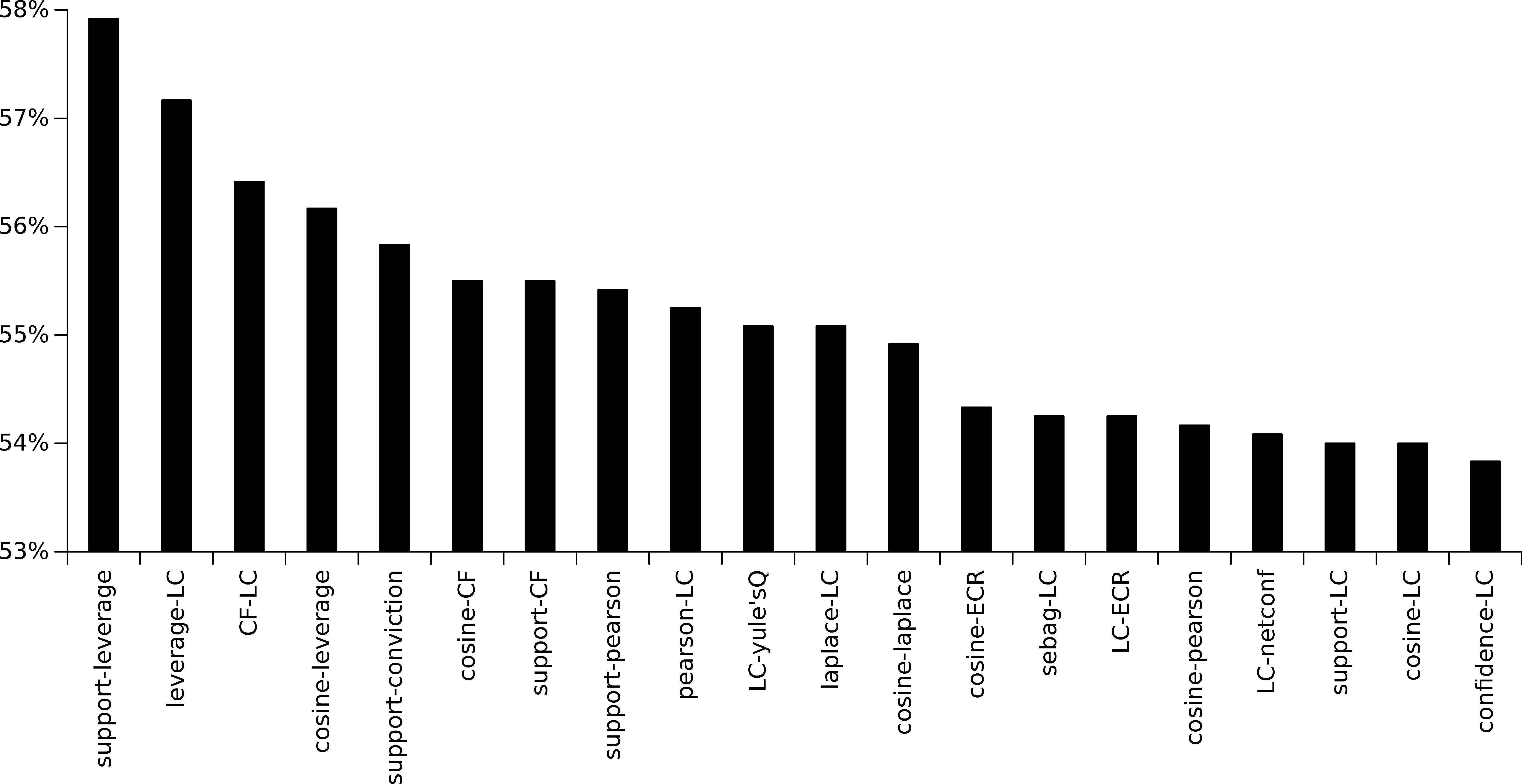
Average percentage of quality measures that was optimized by the best multi-objective functions (those 20 that obtain a best average) and considering the 70th percentile.
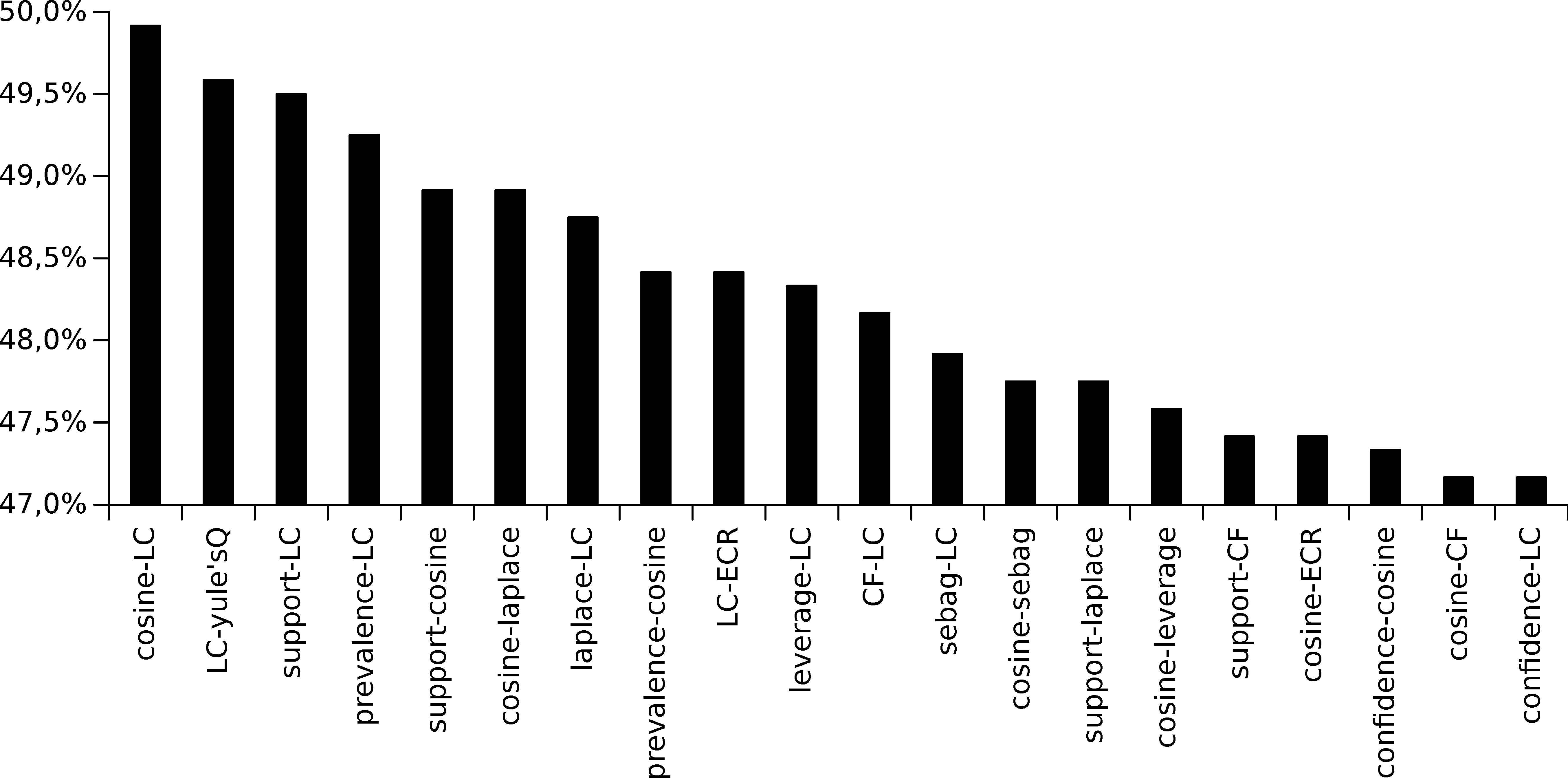
Average percentage of quality measures that was optimized by the best multi-objective functions (those 20 that obtain a best average) and considering the 80th percentile.
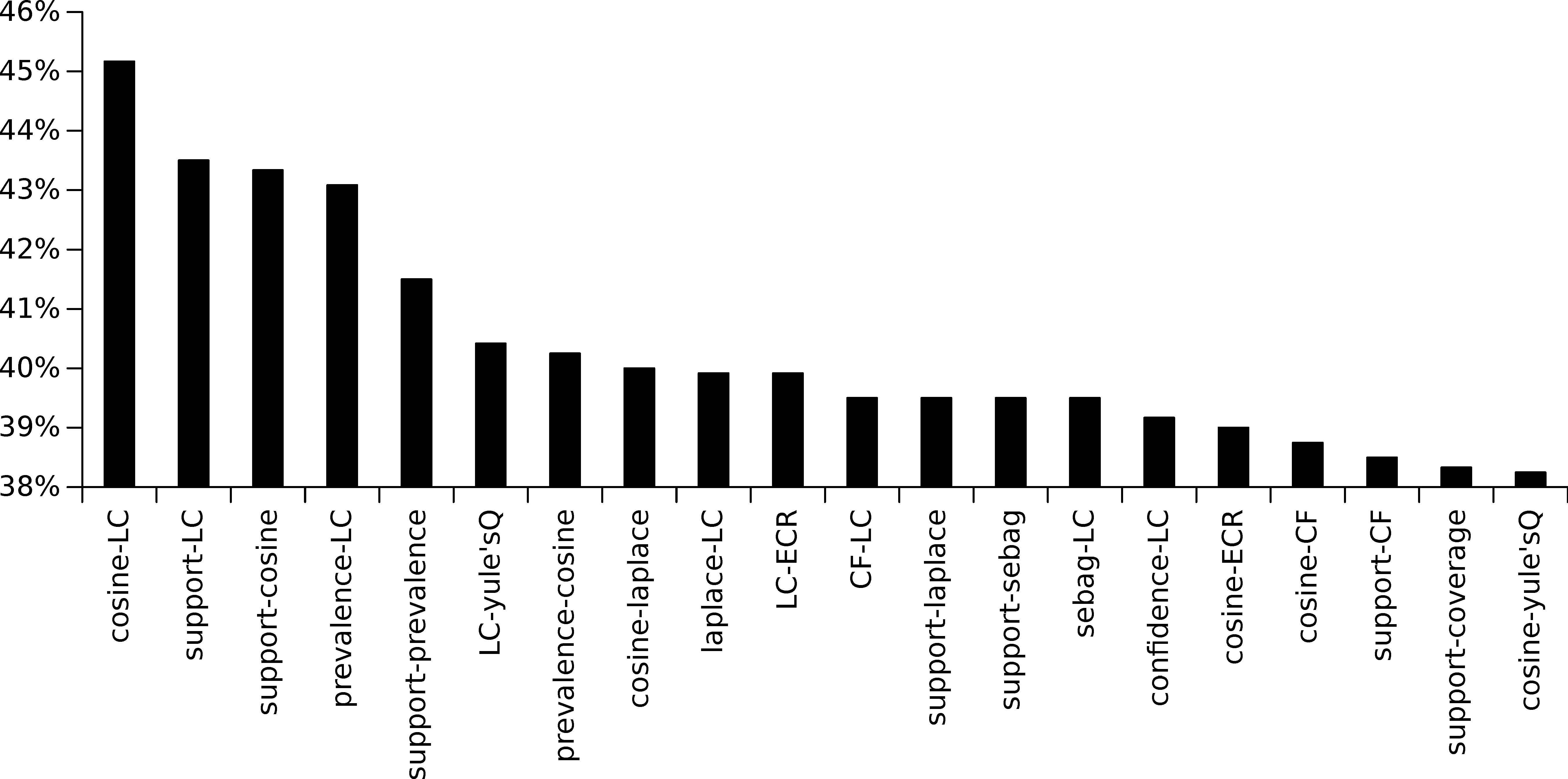
Average percentage of quality measures that was optimized by the best multi-objective functions (those 20 that obtain a best average) and considering the 90th percentile.
Analysing all the results for the three aforementioned percentiles, it is obtained that 14 multi-objective functions appear within the 20 best multi-objective functions for each percentile. These multi-objective functions are the following: Cosine-LC, LC-yule’sQ, Support-LC, Prevalence-LC, Support-Cosine, Cosine-Laplace, Laplace-LC, LC-ECR, CFLC, Sebag-LC, Support-CF, Cosine-ECR, Cosine-CF, and Confidence-LC. When analysing each single quality measure (from the set of multi-objective functions), it is obtained that LC appears in 9 of these 14 multi-objective functions; Cosine in 5 of the 14 multi-objective functions; CF and Support in 3; Laplace and ECR in 2 of the multi-objective functions; and, finally, Prevalence, Confidence, Sebag and yule’sQ in 1 of the aforementioned functions.
Third analysis.
The final analysis is conducted to determine which set of multi-objective functions should be used to maximize the whole set of quality measures. It is based on the percentage of datasets in which each quality measure is marked as optimized when the 70th percentile is considered as shown in Table 7. Due to space limitations, only those multi-objective functions that optimizes a higher number of metrics are shown in Table 7. Among all of them, the first five multi-objective functions are the ones that optimize a higher number of metrics (9 in total). Analysing the results, it is obtained that, when considering Support-Prevalence as multi-objective function, the following metrics are also maximized: Support, Coverage, Prevalence, Confidence, Cosine, Recall, Laplace, LC and ECR. All of these quality measures were optimized in almost all the datasets (>90% of the datasets). The same set of quality measures were also maximized when considering Support-Cosine, Support-Laplace, Support-LC (among others) as multi-objective functions. Hence, taking Support-Prevalence as a multi-objective function, it is required to choose another multi-objective function that maximizes those of quality measures that were not maximized by the previous one. For instance, if we take Confidence-CC as multi-objective function, the following metrics are maximized (those that were not maximized yet): CC, CF, Zhang and Yule’sQ. Finally, it should be noted that the rest of quality measures that were not maximized by any multi-objective function, denoting that they are really hard to be optimized from a multi-objective point of view. As a matter of example, let us focus on the Lift quality measure which takes extremely high values in some datasets. Even when a multi-objective approach enables the maximum feasible value to be obtained, the fact of optimizing more than one quality measure produces a deterioration in the average values of the output. Hence, some quality measures such as Lift, Conviction, Pearson, IG, etc, cannot maximize the values of the output in multi-objective optimization problems. However, this issue does not imply that they are undesirable quality measures to be used on multi-objective optimization but the opposite.
| Multi-objective function | Support | Coverage | Prevalence | Confidence | Lift | Cosine | Leverage | Conviction | CC | CF | Recall | Laplace | Pearson | IG | Sebag | LC | ECR | Zhang | Netconf | Yule’sQ |
|---|---|---|---|---|---|---|---|---|---|---|---|---|---|---|---|---|---|---|---|---|
| Support-Prevalence | 1.00 | 1.00 | 1.00 | 0.98 | 0.03 | 0.98 | 0.05 | 0.03 | 0.03 | 0.20 | 0.93 | 1.00 | 0.13 | 0.03 | 0.40 | 0.93 | 0.98 | 0.20 | 0.00 | 0.10 |
| Support-Cosine | 0.97 | 1.00 | 0.97 | 0.90 | 0.03 | 1.00 | 0.20 | 0.03 | 0.05 | 0.38 | 1.00 | 1.00 | 0.35 | 0.03 | 0.30 | 0.95 | 0.97 | 0.37 | 0.00 | 0.15 |
| Support-Laplace | 0.95 | 1.00 | 0.97 | 0.97 | 0.03 | 1.00 | 0.13 | 0.03 | 0.03 | 0.55 | 0.92 | 1.00 | 0.25 | 0.03 | 0.27 | 0.92 | 1.00 | 0.52 | 0.00 | 0.13 |
| Support-LC | 1.00 | 1.00 | 0.98 | 0.92 | 0.03 | 1.00 | 0.18 | 0.03 | 0.03 | 0.40 | 1.00 | 1.00 | 0.37 | 0.03 | 0.33 | 0.95 | 1.00 | 0.40 | 0.00 | 0.13 |
| Coverage-Prevalence | 1.00 | 1.00 | 1.00 | 0.97 | 0.03 | 0.97 | 0.03 | 0.03 | 0.03 | 0.12 | 0.97 | 0.98 | 0.07 | 0.03 | 0.35 | 0.73 | 0.77 | 0.12 | 0.00 | 0.07 |
| Support-Coverage | 1.00 | 1.00 | 1.00 | 0.93 | 0.03 | 0.98 | 0.05 | 0.03 | 0.03 | 0.10 | 1.00 | 0.97 | 0.12 | 0.03 | 0.32 | 0.75 | 0.75 | 0.10 | 0.00 | 0.07 |
| Support-Yule’sQ | 0.98 | 1.00 | 1.00 | 0.90 | 0.03 | 1.00 | 0.13 | 0.03 | 0.03 | 0.40 | 0.98 | 0.98 | 0.35 | 0.03 | 0.37 | 0.77 | 0.85 | 0.42 | 0.00 | 0.13 |
| Coverage-Cosine | 0.98 | 1.00 | 1.00 | 0.90 | 0.03 | 1.00 | 0.15 | 0.03 | 0.03 | 0.27 | 1.00 | 0.98 | 0.27 | 0.03 | 0.32 | 0.72 | 0.73 | 0.28 | 0.00 | 0.13 |
| Coverage-Laplace | 0.98 | 1.00 | 0.98 | 0.97 | 0.03 | 1.00 | 0.13 | 0.03 | 0.03 | 0.38 | 0.95 | 1.00 | 0.18 | 0.03 | 0.30 | 0.78 | 0.88 | 0.38 | 0.00 | 0.13 |
| Coverage-LC | 0.97 | 1.00 | 0.98 | 0.87 | 0.03 | 1.00 | 0.13 | 0.03 | 0.05 | 0.33 | 1.00 | 0.97 | 0.32 | 0.03 | 0.28 | 0.68 | 0.72 | 0.33 | 0.00 | 0.15 |
| Prevalence-Cosine | 0.98 | 1.00 | 0.98 | 0.93 | 0.03 | 1.00 | 0.17 | 0.03 | 0.03 | 0.37 | 0.95 | 1.00 | 0.27 | 0.03 | 0.35 | 0.95 | 1.00 | 0.35 | 0.00 | 0.15 |
| Prevalence-LC | 0.98 | 1.00 | 0.98 | 0.95 | 0.03 | 1.00 | 0.17 | 0.03 | 0.03 | 0.35 | 0.93 | 1.00 | 0.28 | 0.03 | 0.33 | 0.95 | 1.00 | 0.33 | 0.00 | 0.15 |
| Confidence-CC | 0.03 | 1.00 | 0.02 | 0.03 | 0.10 | 0.17 | 0.07 | 0.03 | 0.98 | 1.00 | 0.13 | 0.77 | 0.43 | 0.03 | 0.12 | 0.15 | 1.00 | 1.00 | 0.00 | 0.97 |
| Confidence-Netconf | 0.05 | 1.00 | 0.03 | 0.03 | 0.07 | 0.42 | 0.32 | 0.05 | 0.98 | 1.00 | 0.33 | 0.83 | 0.65 | 0.03 | 0.17 | 0.30 | 1.00 | 1.00 | 0.00 | 0.97 |
| Conviction-CC | 0.02 | 1.00 | 0.02 | 0.03 | 0.05 | 0.23 | 0.12 | 0.07 | 0.98 | 1.00 | 0.13 | 0.92 | 0.60 | 0.03 | 0.37 | 0.13 | 1.00 | 1.00 | 0.00 | 0.97 |
| Conviction-Netconf | 0.05 | 1.00 | 0.03 | 0.03 | 0.03 | 0.45 | 0.38 | 0.10 | 0.93 | 1.00 | 0.35 | 0.98 | 0.67 | 0.03 | 0.37 | 0.32 | 1.00 | 1.00 | 0.00 | 0.97 |
| CC-CF | 0.03 | 0.98 | 0.02 | 0.02 | 0.05 | 0.15 | 0.07 | 0.00 | 0.97 | 1.00 | 0.10 | 0.73 | 0.42 | 0.03 | 0.10 | 0.12 | 1.00 | 1.00 | 0.00 | 0.97 |
| CC-ECR | 0.03 | 1.00 | 0.03 | 0.03 | 0.10 | 0.18 | 0.07 | 0.03 | 0.97 | 1.00 | 0.13 | 0.82 | 0.43 | 0.03 | 0.13 | 0.13 | 1.00 | 1.00 | 0.00 | 0.97 |
| CC-Netconf | 0.03 | 0.98 | 0.02 | 0.02 | 0.08 | 0.32 | 0.23 | 0.00 | 0.98 | 1.00 | 0.23 | 0.87 | 0.63 | 0.03 | 0.22 | 0.23 | 0.98 | 1.00 | 0.00 | 0.97 |
| CC-Yule’sQ | 0.03 | 1.00 | 0.03 | 0.03 | 0.10 | 0.15 | 0.07 | 0.03 | 0.98 | 1.00 | 0.12 | 0.72 | 0.45 | 0.03 | 0.13 | 0.12 | 0.98 | 1.00 | 0.00 | 0.97 |
| CF-Netconf | 0.05 | 0.98 | 0.02 | 0.02 | 0.05 | 0.40 | 0.27 | 0.02 | 0.98 | 1.00 | 0.28 | 0.87 | 0.67 | 0.03 | 0.20 | 0.30 | 1.00 | 1.00 | 0.00 | 0.97 |
Average percentage (in per unit basis) of datasets in which each quality measure is optimized for each multi-objective function. The 70th percentile was considered.
3.5. Lesson learned
The results obtained in this experimental analysis are quite useful for any researcher in the association rule mining field, specially those focused on evolutionary computation. The analysis has described which quality measures are related (or unrelated) so they should (or should not) be used at time. Considering Support and Confidence as the basic pillars of any good quality measure2, and knowing that these are the two most widely used metrics in this field, it is essential to use them together with other quality measures that provide any additional information. In this regard, when any existing algorithm for mining association rules considers Support/Confidence as measures to be maximized, the following metrics should be avoided since they are also maximized at time: Coverage, Prevalence, CF, Laplace, ECR and Zhang. Hence, there is no sense to choose any of the aforementioned metrics when Support/Confidence are being maximized.
When an expert (or a random user) needs to maximize a specific metric without using it as objective to be maximized but a different metrics, it is good to know that Confidence, ECR, Zhang, CF and Laplace are those more easily maximized. In fact, more than 60% of the metrics enable these measures to be maximized at time. On the contrary, Support, Lift, Leverage, Conviction, IG, Sebag and Yule’sQ are high independent quality measures since they are hardly maximized by any other single metric. This is a really interesting knowledge since anyone who needs to maximize any of that metrics requires to use them explicitly in the algorithm.
Additionally, the experimental results have revealed that Support and Lift appear as the most promising quality measures to be used as metrics to be maximized in any association rule mining problem. Any algorithm designed to maximize these two quality measures will produce a resulting set of rules where 16 over the 20 quality measures are also maximized. Hence, these two quality measures can be defined as general metrics to be considered by any algorithm in this field. In fact, even when it was tought that Confidence is also a good quality measure in this field, this specific metric is maximized together with Support so the use of both at time might be meaningless for some problems. Finally, it is of high interest for any expert user in the association rule mining field to know that Leverage, Conviction, Sebag and Yule’sQ are not desirable to be used as metrics to be maximized since they only maximize a unique quality measure at time. Thus, these four quality measures should be used only in those cases were they are required to be maximized (no additional maximization is required).
As for the multi-objective optimization problem, the results obtained in this analysis have revealed that Coverage, Laplace and Zhang are maximized by a high number of multi-objective functions so they should not be used by any multi-objective algorithm as metrics to be maximized. Taking a 70th percentile, these quality measures are maximized by more than 80% of the results of the 190 pairs of multi-objective functions available in this study. On the contrary, if user need to know which quality measures are high independent to be included as functions in a multi-objective algorithm, the experimental analysis has revealed that Lift, Conviction, IG and Netconf should not be used if the user needs to maximize a higher number of metrics at time.
Focusing on which pair of metrics are better to be chosen if we want the algorithm to maximize a higher number of metric (among the 20 studied metrics), it is obtained that either Support-Prevalence or Confidence-CC maximize 65% of the metrics analysed in this work. For example, considering Support-Prevalence as a multi-objective function, it is obtained that the following measures are maximized: Support, Coverage, Prevalence, Confidence, Recall, Laplace, LC and ECR. The same set of metrics are also maximized if we consider Support-Cosine for a multi-objective algorithm.
Finally, it is interesting to note that, some quality measures (Lift, Leverage, Conviction, Pearson and Sebag) do not produce a self-maximization when they are optimized together with other metics in a multi-objective optimization algorithm. It is quite interesting knowledge for the expert and it is somehow related to the knowledge previously described since some of these measures were defined as hardly maximized metrics in single-objective optimization. Hence, these metrics should be considered as autonomous metrics (either in single-objective or multi-objective algorithms) and should be studied in isolation for any expert.
4. Conclusion
In this paper we have carried out an empirical study to facilitate the decision about which measure should be selected for each specific goal. An extensive analysis has been performed by considering a set of thirty varied well-known datasets from which association rules are mined over a set of twenty quality measures widely used in literature. A set of exhaustive search models as well as highly promising evolutionary algorithms described in literature have been also used to perform this study, considering either single-objective algorithms and multi-objective optimization approaches. For each algorithm and each quality measure more than 57,000 executions were done. The obtained results are of high interest for future researches on the field, determining which single quality measure (or pairs of them) should be used if other different metrics are required to be optimized.
Acknowledgments
This research was supported by the Spanish Ministry of Economy and Competitiveness and the European Regional Development Fund, project tiN2017-83445-P
References
Cite this article
TY  - JOUR
AU  - J. M. Luna
AU  - M. Ondra
AU  - H. M. Fardoun
AU  - S. Ventura
PY  - 2018
DA  - 2018/11/01
TI  - Optimization of quality measures in association rule mining: an empirical study
JO  - International Journal of Computational Intelligence Systems
SP  - 59
EP  - 78
VL  - 12
IS  - 1
SN  - 1875-6883
UR  - https://doi.org/10.2991/ijcis.2018.25905182
DO  - 10.2991/ijcis.2018.25905182
ID  - Luna2018
ER  -