
Multi-Scale Fuzzy Feature Selection Method applied to Wood Singularity Identification
- DOI
- 10.2991/ijcis.2018.25905185How to use a DOI?
- Keywords
- Image processing; Fuzzy logic; Pattern recognition; Feature selection; Choquet integral
- Abstract
A multi-scale feature selection method based on the Choquet Integral is presented in this paper. Usually, aggregation decision-making problems are well solved, relying on few decision rules associated to a small number of input parameters. However, many industrial applications require the use of numerous features although not all of them will be relevant. Thus, a new feature selection model is proposed to achieve a suitable set of input features while reducing the complexity of the decision-making problem. First, a new criterion, combining the importance of the parameters as well as their interaction indices is defined to sort them out by increasing impact. Then, this criterion is embedded into a new random parameter space partitioning algorithm. Last, this new feature selection method is applied to an industrial wood singularity identification problem. The experimental study is based on the comparative analysis of the results obtained from the process of selecting parameters in several feature selection methods. The experimental study attests to the relevance of the remaining set of selected parameters.
- Copyright
- © 2018, the Authors. Published by Atlantis Press.
- Open Access
- This is an open access article under the CC BY-NC license (http://creativecommons.org/licences/by-nc/4.0/).
1. Introduction
In many pattern recognition problems, the study and the selection of features (or suitable parameters) is fundamental to focus on the most significant data. The feature selection area of interest consists in reducing the dimension of the problem providing many potential benefits according to (Guyon and and Elisseeff., 2003). Among others, it makes the visualization and comprehension of the data easier, reduces the computation time of the classification method (training and use), and reduces the dimensionality in order to improve the accuracy of the classification, and to limit the risk of learned classifiers to over-fitting training data (Yu and Liu, 2004). Feature selection is usually preferable to feature transformation (PCA) when the original units and meaning of features are important and the modeling goal is to identify an influential subset. When categorical features are present, and numerical transformations are inappropriate, feature selection becomes the primary means of dimension reduction. Another way to reduce the complexity is to apply methods reducing the number of features by rules such as FARC-HD (Alcala 2011 and al.,) or FURIA (Huhn and Hüllermeier, 2009). These methods, based on fuzzy associative rules, use an indirect way to decrease the dimensionality of a problem (Han and al., 2006). However, they do not decrease the number of input variables of the system to be computed and then the computation time taken by the extraction step does not significantly come down. A comparison of the proposal method and previous cited ones is given in (Molina and al., 2015).
Thus, this paper focuses on feature selection methods and presents a new model to obtain a convenient set of input parameters, working on a specific industrial context. Langley divided the features selection methods in two groups according to the unsupervised or supervised aspect of the algorithm, respectively named “filter” methods and “wrapper” methods (Langley 1994).
“Filter” methods select from the dataset a subset of features which are independent of the classification algorithm and then can be used with different classifiers. Thus, their computational cost is low, which facilitates their application on huge datasets. This kind of methods takes into account the data structure and the information contained in their spatial distribution. (Ferreira and Figueiredo, 2012), (Guyon and Elisseeff, 2003) use the relationship between input features and output classes. (Liu and al., 2014), (Zhang and Sun, 2002) and (Zhao and al., 2013) consider both, the inter and intra-classes distances in order to preserve the internal structure of data. These criteria are well adapted for processing high dimensional problems which are not our context.
Thus, we focus on the “Wrapper” methods which include a supervised classification to measure the accuracy of the selected subset of features. Despite their high computational cost (Ferreira and Figueiredo, 2012), these methods provide a high discriminative feature subset. Nevertheless, this efficiency is only checked for the used classifier (Guyon and Elisseeff., 2003). The misclassification rate is generally used as selection criterion, generating a high number of tests done on every subset in order to achieve an optimal classification, as it is described in (Chen and al., 2012). The well-known Sequential Floating Search Methods (SFSM) were introduced by (Pudil and al., 1994). Within them, forward methods (SFFS) and backward methods (SFBS), are the most known and used. In (Grandvalet and Canu, 2002) as in (Li and al., 2004) (De Lannoy and al., 2011), a Support Vector Machine method is used as classifier to automatically determine a subset of relevant features. The relevance is measured by scale factors which determine the input space metric, and the features are selected by assigning a null weight to irrelevant features. In (Yu and al., 2011), the relevance or the redundancy of the features is evaluated by using fuzzy mutual information and fuzzy entropy.
Thus, “wrapper” feature selection problem consists in searching an optimized feature subset which aims to maximize the accuracy of the pattern recognition system. Working on a specific industrial context implies many constraints. One main constraint is the necessity to work with not disjointed classes, because of their own fuzziness or of the operator subjectivity. Another constraint is that the system must be able to work with small training datasets often not well-balanced (some singularity classes are rare). The respect of the real-time constraint of the industrial production system is another challenge. Consequently, the recognition model must remain relatively simple and the use of basic operators is required. In other words, the main problems rely both on the amount of data to be processed and on their quality. Moreover, only basic features are calculated (such as perimeters, or surface values) due to the real time constraint. So, it is important in such a context to provide a system, which can efficiently process a few data which can also be vague while keeping the most efficient parameters.
So far, this kind of classification problems is relatively poorly investigated (Abdulhady and al., 2005), (Yang and al., 2002) (Murino and al., 2004). So, this work can be related to the “small scale” domain definition (Kudo and Sklansky, 2000), (Zhang and Zhang, 2002) due to the small number of features.
Working with several classifiers makes it possible to integrate their discriminatory aspects to improve the recognition step (Melnik and al., 2004). Classification methods are generally built separately. Their combination may induce positive interactions, because their goal is to achieve the same result and they are based on the same learning dataset (Littewood and Miller, 1989), (Ho 2002).
The dependence between data is another problem, even if approaches like Adaboost, arcing (Breiman 1996) and boosting (Schapire and al., 1998) try to limit it by reinforcing their diversity. This phenomenon is difficult to measure it in order to efficiently incorporate it into the classification process (Melnik and al., 2004), (Hadjitodorov and al., 2006). Moreover, such methods often require a consistent amount of training data to be efficient (Duda and al., 2001), (Stavrakoudis and al., 2012). A lot of classifier combination has been proposed and compared in the literature (Kittler and al., 1998), (Duda and al., 2001), (Ruta and Gabrys, 2000), (Stejic ad al., 2005), (Jain and al., 2000). A full presentation of most of these can be found in a reference book by (Duda and al., 2001).
For most of the aggregation operators, the relative importance of a feature is represented in the final decision by a weight assigned to the related criterion. However, none of the usual operators, such as quasi-arithmetic means or ordered weighted average (OWA), takes into account the possible interactions between the features to be aggregated. Thus, we propose to use operators based on the Choquet integral which are able to capture the positive or negative synergy of a feature subset in the associated Fuzzy measure (or capacity). Furthermore, Grabisch has proposed an efficient algorithm (Grabisch 1995a) able to learn the Fuzzy measure with scarce data while providing coherent results while avoiding the ill-conditioned matrix problem when the minimization system is solved. Another main interest of such an operator is the possibility to extract both importance and interaction indexes from the capacity and so to quantify the impact of each feature on the final decision.
In (Schmitt and al., 2008) a Fuzzy Rule Iterative Feature Selection (FRIFS) method was proposed. It combined a Fuzzy Rule Classifier (FRC) (Bombardier and al., 2010) and a feature selection from capacity learning by studying a subset of weak parameters at each step. The feature selection method needs a classification step, and the Fuzzy Rule Classifier was chosen because of the industrial specific context (Bombardier and al., 2010) (Schmitt and al., 2009) and to focus on the interpretability of the classification model. Fuzzy rule-based classification systems can provide a good compromise between model simplicity and classification accuracy (Stavrakoudis and al., 2012). Moreover, using a soft computing method in this context of wood singularity identification can be justified. Firstly, the singularities to be identified are intrinsically fuzzy because there is not a crisp transition between sound wood and singularities. The extracted features are thus uncertain despite they are precisely calculated. The use of soft computing method makes it possible to take this into account. Moreover, the definition of the output classes is rather subjective because the boundaries between the classes are not crisp (some kinds of “nodo muerto” can be confused with “nodo suelto”).
The small number of available samples for training and the unbalanced classes can be remedied by the good generalization capacity of the FRC (Schmitt and al., 2008). The major inconvenience of using the Choquet integral lies in the number of features to be considered. According to (Grabisch and Nicolas, 1994), aggregation methods are not efficient enough to process when there are more than ten features. The number of rules highly increases when a great number of features is considered, causing the classifier to behave badly and therefore leading to a bad interpretability.
This paper is outlined as follows. In Section 2, we introduce some background on the Choquet integral, and its use as a multisource aggregation operator. In Section 3, the proposed method to process multiple features is explained. In Section 4 a comparative study using Sequential Backward or Forward Feature Selection methods (SBFS or SFFS) (Pudil and al., 1994) or a Support Vector Machine based method (Grandvalet and Canu, 2002) is carried out to show the efficiency of our method. Finally, in Section 5, we draw conclusions based on these results.
2. Aggregation Based on the Choquet Integral
2.1. Background
The Choquet integral belongs to capacity theory. Let C1, C2, … , Cm, be m output classes and X a set of n decision criteria X={D1, … ,Dn}. A decision criterion is defined from a feature description and an associated metric (usually Jaccard based index). Let x0 be a sample. The goal is to calculate the confidence degree in the statement “According to Dj, how x0 belongs to class Ci”. Let P be the power set of X. A capacity (or fuzzy measure) μ, is defined by:
Fuzzy measures generalize additive measures by considering monotonicity. Let μ be a fuzzy measure on X. The Choquet integral of φ = [φ1, … ,φn]t with respect to μ, denoted Cμ(x), is defined by:
2.2. Training step
The expression of the Choquet integral needs the evaluation of any subset of P(X). Several means to automatically compute the 2n -2 values exist (Grabisch and Nicolas, 1994). The main problem relies on keeping the monotonic property of the integral considering a growing number of sets. Generally, such a problem is traduced to another optimization problem, usually solved by using the well-known Lemke method. M. Grabisch has shown that this kind of approach may induce an inconsistent behavior when a few samples of data are used. He proposed an optimal and efficient gradient-based algorithm (Grabisch 1995a). Such an algorithm tries to minimize the mean square error between the values of the Choquet integral and the expected ones.
It is assumed that without any information, the aggregation is done with the arithmetic mean. Here, a training pattern yields training samples, also called alternatives. Basically, the output is set to 1 (target class) and 0 otherwise. Each fuzzy measure is learned using a gradient descent algorithm with constraints. Considering the Choquet intregal value calculated from a training set of alternatives and the expected one assumed to be an ideal measure, this method tries to minimize the mean square error between both values.
For a training sample, the parameter vector is the current value of the fuzzy measure along the path set by the ordering of the training vector values. The lattice shown Fig. 1 is a suitable representation of the fuzzy measure coefficients. The parameter vector is expressed along the gradient direction with a magnitude proportional to the error, thus updating the values along the path.
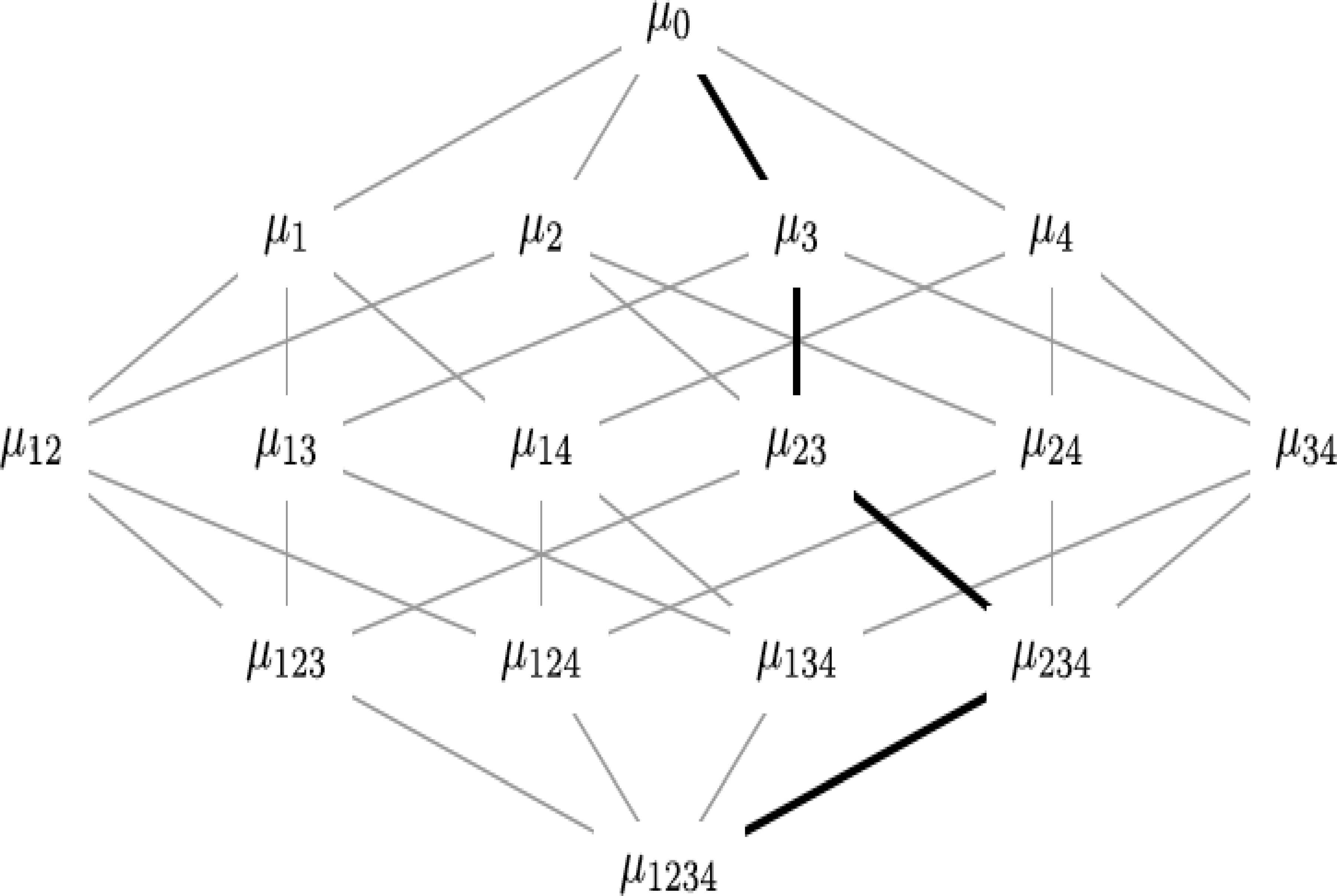
Lattice of the coefficient of a fuzzy measure (n=4) and path μ0, μ3, μ23, μ234, μ1234
2.3. Capacity indices
Once the fuzzy measure is computed, the whole contribution of each criterion in the final decision can be interpreted. In order to analyze the behavior of the decision criteria, we can extract helpful indices from the fuzzy measure, to analyze the behavior of decision criteria (Grabisch 1995b). The significance of each criterion is based on Eq. (3) proposed by Shapley in the game theory (Shapley 1953).
The Shapley index depends on a weighted average value of the marginal contribution μ(T∪i) − μ(T) of Di alone in all combinations. Furthermore:
The interaction index, also called the Murofushi and Soneda index (Grabisch 1995b) (Murofushi and Soneda, 1993) assesses the positive or negative degree of interaction between two decision criteria.
Eq. (4) gives the interaction between Di and Dj, conditioned to the presence of combination elements T ⊆ X\Di,Dj.
After averaging it over all the subsets of T ⊆ X\DiDj the assessment of the interaction index of Di and Dj, is defined by:
And so on to consider any pair (Di,Dj) with i ≠ j. Obviously the indices are symmetric, i.e. I(μ,DiDj)=I(μ,DjDi).
A negative interaction index implies that the sources are antagonistic. Otherwise a positive interaction index between Di and Dj means that the second criterion enhances the decision provided by the first one.
3. Multi-Scale Feature Selection
3.1. Description of the system
The method can be divided into two main steps (see Fig. 2). First, a parameter selection model is defined by studying the impact of both the weakest and highest parameters in subsets. To do so, new combinations of index measures, called here MS1 and MS2, are introduced to rank parameters according to their importance. Only the weakest parameter is processed instead of a subset of usually two or three weakest parameters as in previous FRIFS algorithm. Then we propose an algorithm able to process a larger number of parameters by partitioning them into readable subsets without using the classification step. A parameter selection model is defined by studying the impact of both the weakest and highest parameters in the subsets. The removing criterion is only based on parameter ranking instead of an assessment of recognition rates, as in (Schmitt and al., 2008) for instance.
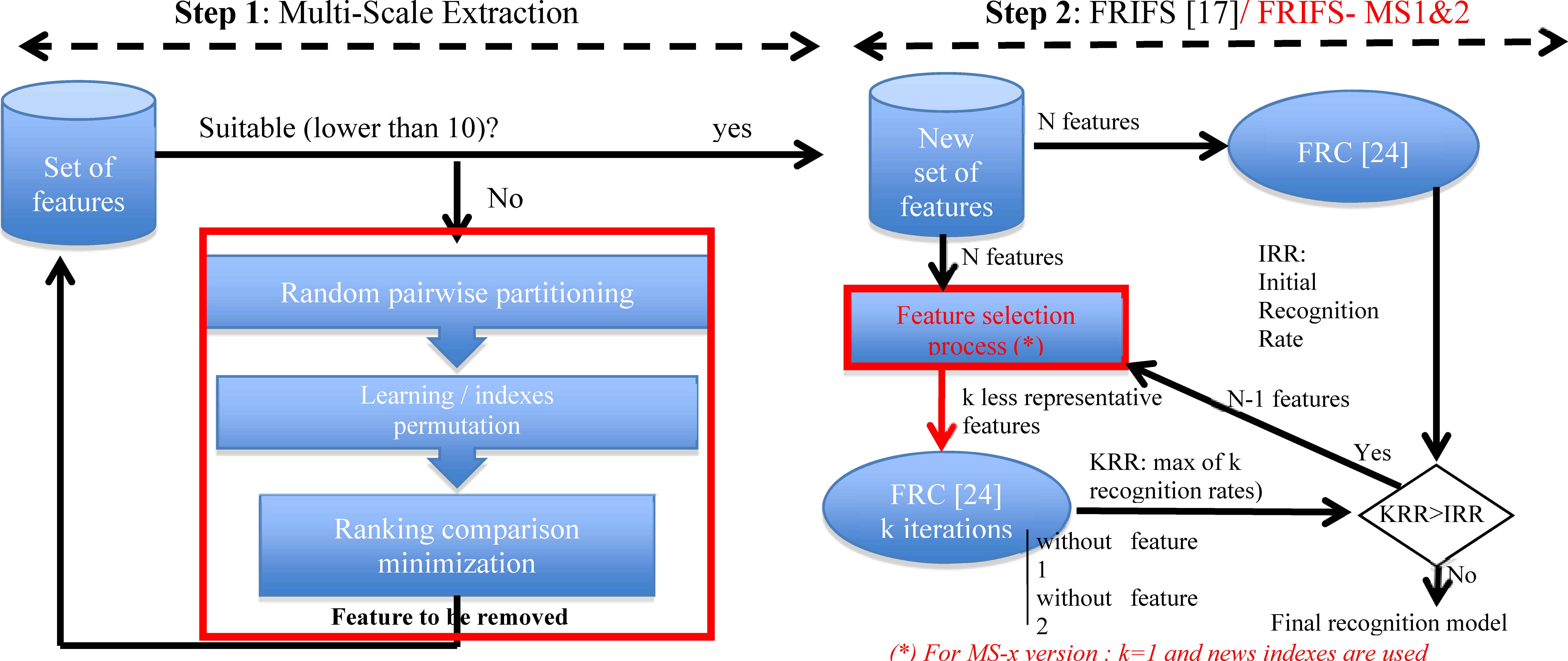
Details of the two steps of the Feature Selection Method
In the second step, the FRC is applied when the size of the remaining set is satisfactory. The system is set up from this new set of features and a global recognition rate is obtained. Here we consider three approaches: on the one hand the classical FRIFS method previously described in (Schmitt and al., 2008) and applied as follows. The identification model is learned and tested, without the least significant features (Fig. 2 - step2). The reached accuracy value is stored. The process is iterated using the k next least significant features. Whenever a better score is reached, the weak feature is removed and so on until no recognition rate improvement is obtained. On the other hand, we also propose two other new strategies, namely FRIFS-MS1 and MS2, to avoid building and testing numerous systems associated to k iterations. Only the weakest one calculated from new proposed criteria, is processed (that is with k=1) in order to provide a faster iterative step.
In section 4, the proposed method is applied to an industrial wood singularity identification problem by studying the sets of parameters obtained at different steps. This application is used to compare different feature selection methods. The comparison is done according to the classification rate. However, the idea is not to compare classifiers but to show the impact of the remaining set of parameters, compared to other feature selection methods widely used.
3.2. Weakest decision criteria
Once the lattice is learned (see section 2.2), the single significance of each Di in the provided fuzzy measure is analyzed (Rendek and Wendling, 2006). The decision criteria are sorting with an increasing order. This is done by using a linear combination between importance degree (Shapley index) and interaction indexes.
A normalization factor K is defined from the average impact of order 2 interactions as shown in Eq. (6).
If the value of K is weak (K ≈ 0), we can directly assume that there are no (or few) interactions between the decision criteria, and that they are independent. In such a case the Choquet integral can be assimilated to a weighted sum. So, the significance of each decision criterion can be estimated by taking the Shapley values fDi = σ(μ,Di).
Otherwise, the importance and the interaction indices are essential and should be assessed as shown in Eq. (7). The interaction impact of Di is determined as follows:
The M value represents the whole interaction reached by one decision criterion. The decision criterion having the least influence on the final decision and interacting the least with the other criteria is assumed to blur the final decision.
3.3. Multi-scale extension
As bad behavior may occur when aggregation methods are used to process with more than ten criteria (Grabisch and Nicolas, 1994), we propose a new approach which aims to iteratively decrease the number of criteria until the set can be interpreted by using the vanilla FRIFS version.
The first step of the method randomly splits X into N subsets Xi, such that
For each Xi, a training step is performed on each associated capacity μi using the Grabisch’ algorithm. Then, Eq. (7) is calculated to sort out the decision criteria of the N capacities by increasing impact.
Let us consider two subsets Xi and Xj with i≠j. Both weakest and highest decision criteria are permuted between each subset. A new training step is then performed and a new ranking of decision criteria is provided for X’i and X’j. If one (or two) permuted decision criterion is set to be weak again, it is removed from X.
If zero decision criterion is extracted from any pair, then the weakest decision criterion, considering the N subsets, is removed from X to ensure the convergence of the algorithm. This step is iterated until a “good” sized set of features is obtained. An overall description of the algorithm is given below.
While minimization is being performed
- Random partitioning of X into N subsets Xi
For each Xi,
- Training of capacity (Fuzzy measure) μi
- Decision criterion ranking
End for each
- Random choice of pairs (Xi,Xj)i≠j describing X
For each (Xi,Xj)
- Permutation 2 ⇔ 2 weakest and highest decision criteria
- New training of μ’i, μ’j / new ranking
If one (or two) decision criterion is set to weak
again then Remove it (them) from X
End for each
If no decision criterion was previously removed then
- Consider the N subsets and remove the weakest
decision criteria from X
End if
End While
3.4. Lattice path training: some remarks
The more the alternatives, the more lattice paths are taken into account. As real data are used, it is not easy to consider all the paths of the lattice. Consequently, paths can be similar for different alternatives and can introduce error oscillations for identical values of output. The basic algorithm is proved to converge if it is repeatedly trained with the same input data. However, it is not required to attain this convergence, because the fuzzy measure will likely be overfitted to the training set. Thus, it will not be extensive enough to fully represent the classes. In order to have a faster processing, we propose to train the lattice with median values of samples. Such filtering guarantees a good behavior of the algorithm with regard to the convergence following a subset of possible paths but it not warrants a full convergence. As real data are used, it is not easy to consider all the paths of the lattice. The values of the not taken paths are modified (Grabisch 1995a) to check the monotonicity of the lattice, by considering both the fathers and children of the current nodes. Experimentally we process with about 100 epochs and keep the lattice providing the weaker error considering the whole dataset.
We propose in the next section to study two Multi-Scale versions of training steps. The first one, called FRIFS-MS1, is based on the presented training method and the second one, based on redundant path removing, is called FRIFS-MS2
4. Feature Selection Application in a Wood Singularity Recognition context
This study takes place in the context of a company-university collaboration. The proposed feature selection method was checked and compared on real wood data provided by our industrial partner. In this section, the applicative singularity recognition system is first described. Then, the FRIFS-MS enhancements were compared with the original FRIFS method and three other feature selection methods. The comparison is based on the analysis of the singularity recognition rates obtained with the set of selected parameters. The influence of the chosen classifier was also checked. And finally, the relevance of the proposed methods FRIFS-MS1 and 2 was highlighted considering other defect datasets from the same wood specie but also from different species.
4.1. Industrial context description
The objective of this application is to develop a pattern recognition system for wood singularity identification in wood boards. Linear sensors are applied to a combined way to acquire images of the four sides of the wood pieces. Laser sources are used to set the profiles, the orientation of fibers (scatter effect), and the red and infrared intensities. These four components provided by the sensors are sampled at 2 kHz and quantified with a 256-level grey-scale.
The segmentation stage of the image processing system aims to extract defects areas from sound wood and a set of features is computed on the achieved regions in order to characterize the wood singularities (Fig. 3). These features are used to estimate the quality of the final products on production lines. Their speed varies between 200 to 500 meters per minute with a maximum of 100 singularities per meter.
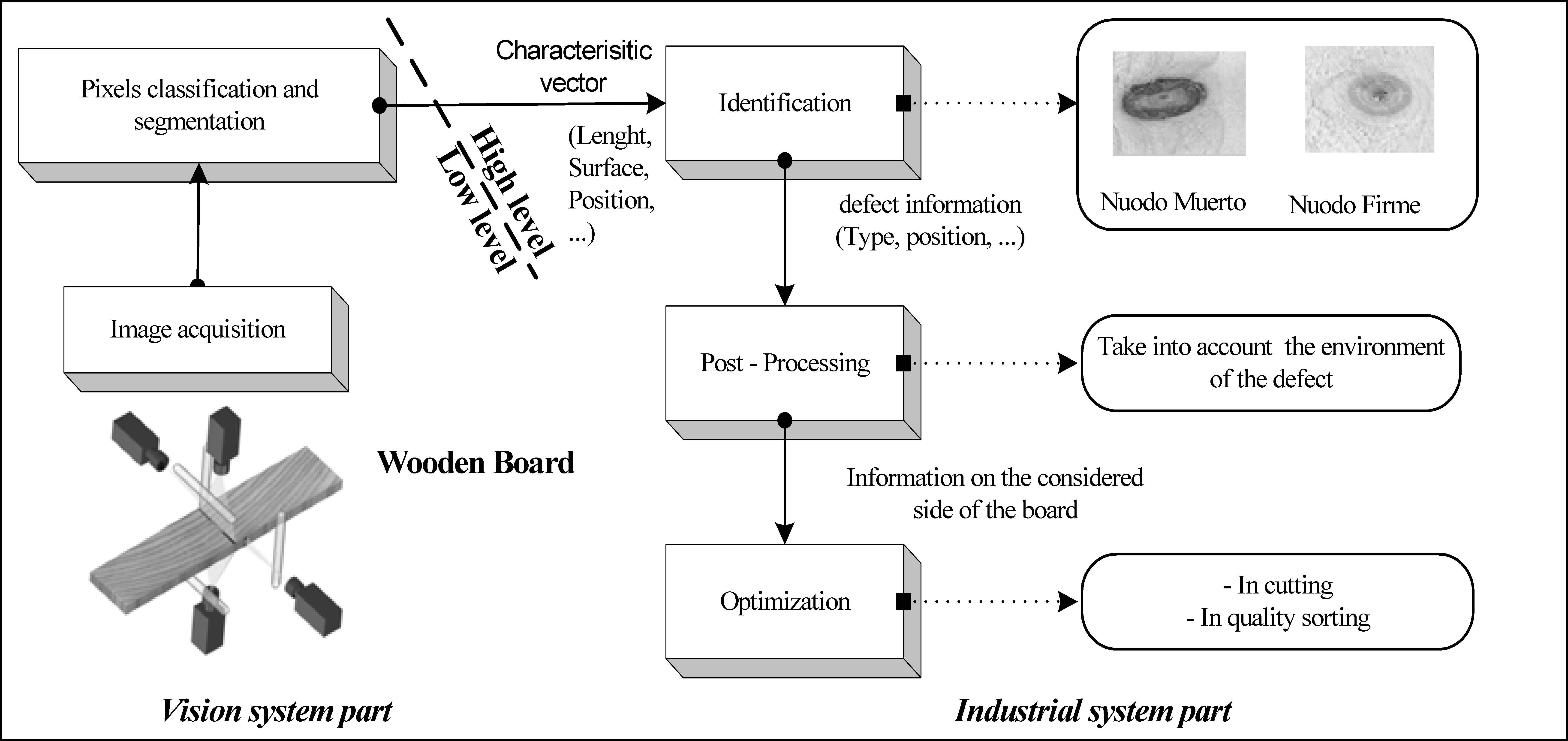
Functioning principle of the vision system. The part named “low level” deals with the acquisition of the wood board images thanks to the different sensors and the first step of image processing (signal processing). The “high level” part concerns information processing from defect identification to board optimization.
The extracted feature set is composed with more than twenty geometrical such as area, major axis, boundary rectangle and topological features. The real-time industrial constraints impose to only extract simple and fast computing feature which are redundant, often contradictory and possibly bring noise to the final decision. The feature selection method relates to the identification stage located in the high level of the image processing system illustrated in Figure 3. The manufacturers usually work with more than twenty basic features without knowing whether they are suitable. We propose to use our feature selection method to reduce this characteristic vector in order to improve the recognition rate and to reduce the model complexity.
The databases used to apply and validate our method are provided by the manufacturer. They are constituted with samples of real singularities named by a human operator. More than 20 features are computed by the low-level step of the vision system. The first database DW1 contains 877 samples issued of nine classes of wood singularities (nudo muerto, nudo suelto, peca, medula, resina …). This DW1 database is relatively heterogeneous and the nine classes are not well balanced. This database was divided into two sets. The first, called “training set”, contains 250 samples (1/3) and the second one, called “generalization set”, is made up of 627 samples (2/3). All the results presented in the following section were obtained with the cross-validation method. The training rates are the mean of the three rates calculated on three permutations of the training database. The same method is applied to compute the generalization accuracy.
4.2. Feature selection evaluation on global singularity recognition
Tests are performed to decrease the dimensionality of the input space by suppressing non-relevant features until an interpretable model is reached while keeping an “acceptable” accuracy. The suitability of the parameter sets was assessed through the singularity recognition rate. This recognition rate was obtained by using the Fuzzy Rule Classifier (FRC) included in the FRIFS method (Schmitt nad al., 2008).
The fuzzy recognition module can be decomposed into three parts. The first step is the Fuzzification of the input features, then the Fuzzy Rule Generation and finally the Rule Adjustment. The Max – Product inference mechanism applies a conjunctive rule set (Dubois and Prade, 1992 & 1996) using the Larsen model (Mendel 1995). The iterative Ishibushi method (Ishibushi and al., 1992 & 1997) is used to automatically generate each rule. The delivered rule set is used to classify the unknown samples and the output class is determined by the rule of maximal answer. For more explanation about the Fuzzy Rule Classifier, readers can refer to (Bombardier and al., 2010) and (Schmitt and al., 2009).
Six feature selection methods are used SBFS, SFFS (Pudil and al., 1994), SVM (Grandvalet and Canu, 2002), vanilla FRIFS method and the proposed extensions FRIF-MS1 and FRIF-MS2.
These methods, except FRIFS, are applied on the industrial database DW1 using, at the beginning, more than 20 features as input of the recognition system. They almost provide the same set of 10 remaining features. The recognition accuracy reaches 94% for training and 74.5% for the generalization tests except for SVM where two features differ (93.6% and 71%). The results provided by applying the feature selection methods on the 10 remaining parameters are different. We compared the efficiency of the feature set provided by the methods with the classification accuracy: Tg.
Table 1 shows the different levels and gives the accuracy Tg obtained with the remaining features according to the removed feature at each level. The successive suppression of parameters is stopped when the training accuracy decreases below 90%. This limit is reached with 8 (SVM) or 4 (FRIFS) features ensuring a good interpretability of the model. The generalization accuracy is given for the last level. It can be seen that the initial FRIFS Method gives the best results. But the generalization accuracies obtained with the other methods are acceptable too. Down to five parameters, FRIFS-MS1 yields results similar to those of the other methods (72.25%) and results are close to those of the vanilla FRIFS method (76.24%), while a supplementary iterative step is required (Fig. 2).
| #Features / Methods | FRIFS-MS1 | FRIFS-MS2 | FRIFS | SBFS / SFFS | SVM | |
|---|---|---|---|---|---|---|
| 10 | Training Accuracy | 94.00% | 94.00% | 94.00% | 94.00% | 93.60% |
| Generation Accuracy | 74.48% | 74.48% | 74.48% | 74.48% | 71.00% | |
| 9 | Removed Feature | LR_RE | LR_RE | LR_RE | LR | CR3 |
| Training Accuracy | 95.20% | 95.20% | 95.20% | 92.00% | 93.60% | |
| 8 | Removed Feature | SURF | MAJ_AXIS | SURF | MAJ_AXIS | ORIENT |
| Training Accuracy | 95.20% | 95.20% | 95.20% | 92.00% | 95.20% | |
| 7 | Removed Feature | C3 | MIN_AXIS | C3 | DX/DY | LR |
| Training Accuracy | 94.40% | 94.00% | 94.40% | 90.40% | 87.60% | |
| 6 | Removed Feature | C4 | C3 | MAJ_AXIS | C3 | C3 |
| Training Accuracy | 84.00% | 93.20% | 93.60% | 90.00% | 88.00% | |
| 5 | Removed Feature | MAJ_AXIS | C4 | MIN_AXIS | SURF | SURF |
| Train. Accuracy | 82.00% | 76.90% | 92.40% | 84.80% | 88.00% | |
| Generation Accuracy | 72.25% | 69.86% | 76.24% | 71.93% | 76.40% | |
| 4 | Removed Feature | MIN_AXIS | DX/DY | C4 | MIN_AXIS | DX/DY |
| Training Accuracy | 80.80% | 74.80% | 80.80% | 74.80% | 75.60% | |
| Gener. Accuracy | 72.41% | 68.90% | 72.41% | 69.86% | 69.38% | |
Evolution of the global accuracy Tg in relation with the number of features. (SBFS and SFFS results are the same and grouped in one column).
However, because the classes are badly balanced, a high accuracy do not provide a satisfactory singularity identification for the manufacturer.
In order to address the manufacturer aim, we used the index Mc which represents the means of each class accuracy Tc (Eq.8). It gives some information about the precision of each class recognition:
This index was calculated with the training data set, because it aims at showing that a “high” Tg does not really mean a good classification. Therefore, it will be better to consider the Mc index to choose the best feature set or feature selection method.
Table 2 provides the Mc values obtained with the selected set of parameters for each method at the different levels. Following this criterion, this shows that our methods are well suited for feature selection in the case of an unbalanced data input. If we consider the same limit for the learning rate (not below 90%), it would be interesting to keep six parameters using FRIFS or seven /eight parameters for other feature selection methods.
| Method \ #Feature | 3 | 4 | 5 | 6 | 7 | 8 | 9 | 10 |
|---|---|---|---|---|---|---|---|---|
| FRIFS – MS1 | 75.41 | 75.94 | 79.39 | 83.27 | 90.99 | 95.43 | 95.43 | 93.44 |
| FRIFS – MS2 | 41.88 | 69.18 | 74.00 | 86.66 | 90.47 | 95.56 | 95.43 | 93.44 |
| FRIFS | 66.56 | 75.94 | 84.32 | 91.16 | 90.99 | 95.43 | 95.43 | 93.44 |
| SBFS/SFFS | 33.30 | 44.40 | 76.68 | 86.47 | 89.86 | 92.14 | 92.14 | 93.44 |
| SVM | 71.20 | 71.20 | 88.96 | 88.99 | 88.87 | 95.56 | 94.52 | 94.52 |
Comparison of the training accuracy (Mc) in relation with the number of features. (SBFS and SFFS results are the same and grouped in the same line).
4.3. Influence of the chosen classifier on the classification rates
The generalization accuracy is used to compare the relevance of the remaining set of features obtained with each method. Such assessment is pointed out by the manufacturer: the required suitable features are those that yield the best recognition accuracy. The aim of these tests is not to compare the classifiers to each other, but rather to study the influence of the selected parameters on the recognition rate, in relation with the chosen classifier. The aim is to show that the efficiency of the feature selection method does not depend on the classifier. The features provided as input of the recognition system are the same for each classifier. The selection is done with the FRIFS method.
The comparison results are made with different families of classifiers. The FRC classifier we used in the FRIFS method (Bombardier and al., 2010) was compared with other well-known classification methods. Usual methods such as Bayesian classifier, k Nearest Neighbors (k-NN) and its fuzzy version (Fuzzy K-NN) or Decision Tree (DT) are chosen. The Support Vector Machine (SVM) classifier is used because it is a reference in pattern recognition. Then, we also test Neural Networks (NN) because this kind of classifier is the most used in the wood industry. We include also the results given in (Molina and al., 2015) which are obtained with the FARC-HD fuzzy associative rule classifier (Alcala and al., 2011).
Table 3 shows the obtained accuracy Tg. It is computed on the whole database, independently of the classes. Several tunings have been checked for each classifier. Only the one giving the best results is presented. For Nearest Neighbor methods, 3, 5 and 7 neighbors have been used and k=5 gives the best accuracy. So, 3 hidden layers and 20 neurons per layer for the Neural Networks classifier are retained. Then, we use trapezoidal membership functions with 5 terms for the FRC. In this case, the configuration is not the best and the reader can refer to (Bombardier and al., 2010) to see the effects of the term number and the form of the membership functions.
| Method \ #Feature | 3 | 4 | 5 | 6 | 7 | 8 | 9 | 10 |
|---|---|---|---|---|---|---|---|---|
| 1Bayesian Classifier | 41.15 | 46.09 | 45.45 | 46.89 | 48.17 | 48.96 | 49.60 | 48.96 |
| 2k-Nearest Neighbor | 71.77 | 73.05 | 75.76 | 76.71 | 77.03 | 79.43 | 78.15 | 67.94 |
| 3Fuzzy k-Nearest Neighbor | 68.90 | 72.25 | 77.03 | 77.99 | 78.47 | 79.11 | 78.63 | 69.06 |
| 4Neural Network | 73.37 | 73.37 | 75.44 | 74.80 | 74.00 | 79.27 | 77.19 | 71.17 |
| 5Fuzzy Rule Classifier | 71.61 | 75.41 | 76.24 | 75.44 | 75.76 | 75.28 | 75.12 | 70.97 |
| FARC-HD Classifier | - | - | 74.50 | 75.60 | 73.40 | 74.20 | 73.20 | 73.40 |
| 6Support Vector Machine | 56.78 | 65.71 | 64.27 | 67.15 | 67.30 | 68.42 | 74.48 | 66.99 |
Classifier tuning: 1 Euclidean distance, 2,3 k=5, 4 hidden layers=3, neurons/layer=20, 5 #terms=5 (regularly distributed), 6 Gaussian kernel.
Generalization Accuracy Tg obtained with different classifiers using the same set of features selected with FRIFS method.
Accuracy varies from 73.4% with 10 features to 73.37% with three features. A maximum of 79.43% is reached with eight features using the k-NN classifier.
These results are quite similar despite the fact that the fuzzification step of FRC is not optimized such as shown in (Schmitt and al., 2007). However, such recognition accuracy is not significant because it considers the whole database even though the number of samples is not equal for each class. The rate of 79.27% is only reached with NN when almost all the samples of the classes having the greatest number of samples are recognized. Nevertheless, we can see that all the classifiers have the same behaviour except for the Bayesian and to a lesser degree the SVM that are not well suited to the industrial context. Conversely, the soft computing classifiers (NN or Fuzzy Classifiers) give the best results. It can be noted that the FRC and FARC-HD classifiers give the best results with the least number of features (respectively 5 and 6). This shows the generalisation capabilities of fuzzy operators and that the Fuzzy Logic is well adapted to this industrial context.
To avoid the classifier influence, an efficient “classifier-free” index Ic (Eq. 9) is computed to give a compromise between the index (Mc) and the standard deviation (Sd) of the accuracy Tc for each class and the global accuracy Tg. Ic is computed from the results given by all the previous classifiers applied to the same specific set of features as shown in (EQ.9).
Figure 4 shows the variability of Ic for each feature selection method. The goal is to limit the impact of the classifier in order to determine the best feature set and consequently, the more efficient feature selection method.
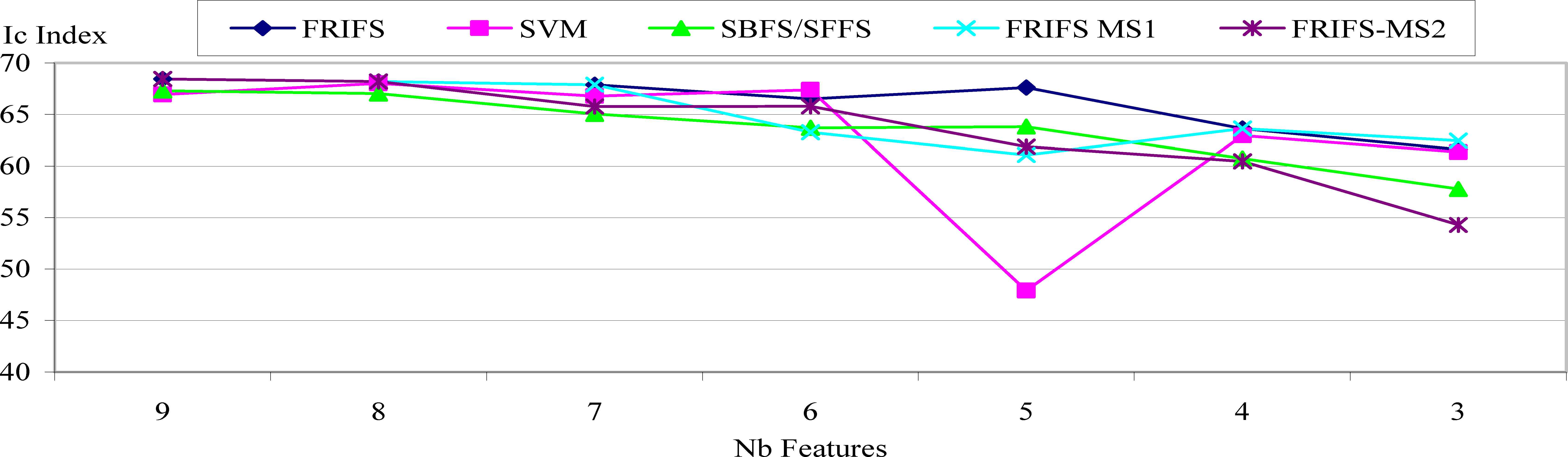
Mean of all classifier indexIc calculated for each feature selection method (SBFS and SFFS results are the same and grouped).
Depending on the application, the remaining features depend also on the selection method. Nevertheless, they refer to the same kind of information (size, shape, color…) even if they are not equal (DX/DY ratio for one method, compactness index for another). In most cases FRIFS yields the best results, which is coherent with other application contexts based on fibers (Schmitt and al. 2008). FRIFS-MS1 is the improved method that gives the results closer to the optimal set of features, but FRIFS-MS2 provides very similar results while requiring fewer learning samples.
4.4. Generalization test on other Dataset with the same tree species
Other datasets, DW2 and DW3, consisting of samples issued from the same tree species were used to check the selected features. These datasets are respectively composed of 311 samples (80 for learning set, 231 for generalization set) and 1042 samples (134 for learning, 908 for generalization). They are taken from two different sensors: DW2 is defined using sensors RIGHT/LEFT and DW3 is defined using sensors TOP/BOTTOM (see figure 3). Different segmentation step adjustments yielded more features. The results obtained for DW1 by using six and seven parameters considering the best configuration for each method are provided in table 4.
| Data Sets | Data Set DW2 | Data Set DW3 | ||||||
| 6 features | Learn rate | Gene rate | Mc | Ic | Learn rate | Gene rate | Mc | Ic |
| FRIFS | 91.25 | 69.70 | 55.23 | 66.48 | 90.30 | 73.79 | 59.36 | 69.62 |
| FRIFS-MS1 | 91.25 | 74.03 | 59.04 | 65.50 | 81.34 | 70.49 | 55.09 | 65.24 |
| FRIFS-MS2 | 91.25 | 69.26 | 49.39 | 63.50 | 85.82 | 67.40 | 52.32 | 64.98 |
| SFFS/SBFS | 91.25 | 71.86 | 54.50 | 65.86 | 85.08 | 73.02 | 56.29 | 66.73 |
| SVM | 91.25 | 76.19 | 51.49 | 66.06 | 89.55 | 71.81 | 55.49 | 66.80 |
| Data Sets | Data Set DW2 | Data Set DW3 | ||||||
| 7 features | Learn rate | Gene rate | Mc | Ic | Learn rate | Gene rate | Mc | Ic |
| FRIFS | 92.50 | 75.33 | 58.16 | 68.74 | 91.05 | 72.47 | 57.00 | 68.85 |
| FRIFS-MS1 | 92.50 | 75.33 | 58.16 | 68.74 | 91.05 | 72.47 | 57.00 | 68.85 |
| FRIFS-MS2 | 90 | 69.26 | 50.16 | 63.88 | 89.55 | 68.06 | 52.87 | 65.12 |
| SFFS/SBFS | 90 | 71.43 | 53.76 | 65.61 | 82.84 | 73.68 | 56.40 | 66.72 |
| SVM | 91.25 | 74.89 | 49.60 | 65.39 | 89.55 | 74,12 | 55.49 | 67.01 |
Classification rates obtained with DW2 and DW3. (SBFS and SFFS results are the same and grouped in one row).
It is worth noting that the remaining feature sets are coherent because the achieved classification is quite similar to those obtained with DW1. Indices Mc and Ic show that the FRIFS method remains the most discriminative with regards to the classes even if associated mean recognition rates are not always better. FRIFS-MS1 and MS2 also have a good behavior on these datasets.
4.5. Tests on another tree species
The aim of this new series of tests is to show the genericity of the proposed methods. Here another dataset of species, denoted by DW4, is processed. This dataset is composed of 133 samples for the learning step and of 192 samples for the generalization step. The number of output classes (9) is the same as that of DW1, DW2 and DW3, but the defects are quite different. The system segmentation step differs too. Thus, the experimental results show that previous feature sets are not relevant and produce bad results with generalization rates lower than 60%. Then new sets were performed from the initial set which is composed of more than 20 features. A remaining set of nine features was selected using six methods (FRIFS, FRIFS-MS1, MS2, SBFS, SFFS and SVM). For these tests, we added an EXPERT method, which means that the parameters were selected by an industrial expert on the existing recognition system. We did not have this expert selection for the previous study. Table 5 gives the value of the learning and generalization rates, and of the Mc and Ic indexes. When the parameter removing step was stopped the learning rate fell below 90% (i.e. 6 features).
| 9 features | Learn. Rate | Gene Rate | Mc | Ic |
| FRIFS | 90.32 | 71.35 | 66.24 | 74.53 |
| FRIFS-MS1 | 90.32 | 71.35 | 66.24 | 74.53 |
| FRIFS-MS2 | 91.94 | 70.83 | 62.91 | 70.64 |
| SVM/SBFS | 91.94 | 70.83 | 62.91 | 70.64 |
| SFFS | 91.94 | 70.83 | 62.91 | 70.64 |
| EXPERT | 91.13 | 71.88 | 63.61 | 71.11 |
| 8 features | Learn. Rate | Gene Rate | Mc | Ic |
| FRIFS | 91.13 | 72.40 | 67.28 | 74.99 |
| FRIFS-MS1 | 91.13 | 72.40 | 67.28 | 74.99 |
| FRIFS-MS2 | 91.94 | 72.40 | 66.43 | 71.34 |
| SVM/SBFS | 91.94 | 72.40 | 66.43 | 71.34 |
| SFFS | 91.94 | 72.40 | 66.43 | 71.34 |
| EXPERT | 89.52 | 70.31 | 64.38 | 73.79 |
| 7 features | Learn. Rate | Gene Rate | Mc | Ic |
| FRIFS | 90.92 | 75.00 | 71.97 | 77.33 |
| FRIFS-MS1 | 90.92 | 75.00 | 71.97 | 77.33 |
| FRIFS-MS2 | 91.13 | 61.98 | 68.30 | 72.73 |
| SVM/SBFS | 88.71 | 70.31 | 63.67 | 69.66 |
| SFFS | 91.94 | 73.96 | 70.64 | 75.18 |
| EXPERT | 86.29 | 60.94 | 57.59 | 66.81 |
| 6 features | Learn. Rate | Gene Rate | Mc | Ic |
| FRIFS | 92.74 | 73.96 | 70.70 | 77.20 |
| FRIFS-MS1 | 89.52 | 77.08 | 72.72 | 77.82 |
| FRIFS-MS2 | 86.29 | 62.50 | 57.16 | 65.24 |
| SVM/SBFS | 87.90 | 61.46 | 58.06 | 65.17 |
| SFFS | 90.32 | 64.06 | 61.69 | 67.91 |
| EXPERT | 79.03 | 53.13 | 52.59 | 59.01 |
Classification rates, Mc and IC indexes obtained with DW4. (SBFS and SFFS results are the same and grouped in one row).
First it can be noted that the expert does not select efficient parameters. All the feature selection methods provide better results.
We can remark that eight features (out of 10) correspond to those selected by the expert on the existing system. The generalization rate reached using the 10 expert selected features is equal to 72.92%.
Finally, the selected features obtained by using the proposed methods give rise to both better recognition rates and better indices Mc and Ic than those provided by the expert. Table 5 shows that the best results are reached with seven features using FRIFS-MS2 and SFFS (8 for SVM and SBFS). Both selection methods FRIFS and FRIFS-MS1 provide very interesting results when the maximal rates are achieved with six features and the indices Mc and Ic attest to this result.
It can be noticed that removing four features makes it possible to increase the generalization rate up to 4% with the FRIFS-MS1 selected feature set. The set of resulting rules given by the FRC classifier becomes interpretable and can be used very quickly in a real-time context.
5. Concluding Remarks
The aim of this paper is to present an enhancement of a previous feature selection method (FRIFS). This “multiscale” improvement allows to easily process with more than 10 features to be selected. The partitioning of the set of features is performed through the definition of a criterion based on both significance and interaction indices. The basic method was improved by unifying the scanned paths of the capacity, which makes it possible to decrease the learning time and to focus on relevant samples. Finally, the improved automatic selection process makes it easier to use the method in an industrial context.
Such algorithm makes it possible to efficiently decrease the number of features until providing an interpretable dataset to be used with a Fuzzy Rule Classifier (Bombardier and al., 2010). This method is robust and the remaining sets seem to be relevant according to several classifiers. Furthermore, Mc and Ic indices attest of the good behavior of our method, which aims at providing remaining features, representative of all the classes. Tests performed on several industrial databases confirm the interest of reducing the number of features while both increasing the recognition rate and improving the interpretability of the system. Results obtained in this wood industry context with four different databases underline the generic aspect of the method. Although our study involved a larger number of parameters, results are in agreement with those previously obtained in a fabric pattern recognition context (Schmitt and al., 2008). The overall accuracy is better than the one provided by using the feature set selected by other methods and the accuracy is also better for each class. The vanilla FRIFS method and the proposed Multi-Scale evolvement attest of its efficiency in the case of small and non-balanced data sets.
Further works will be done to extend our method to select features per class in order to be able to automatically create a hierarchical classifier (Molina and al. 2015).
References
Cite this article
TY  - JOUR
AU  - Vincent BOMBARDIER
AU  - Laurent WENDLING
PY  - 2018
DA  - 2018/11/01
TI  - Multi-Scale Fuzzy Feature Selection Method applied to Wood Singularity Identification
JO  - International Journal of Computational Intelligence Systems
SP  - 108
EP  - 122
VL  - 12
IS  - 1
SN  - 1875-6883
UR  - https://doi.org/10.2991/ijcis.2018.25905185
DO  - 10.2991/ijcis.2018.25905185
ID  - BOMBARDIER2018
ER  -