
Fuzzy Rough Graph Theory with Applications
- DOI
- 10.2991/ijcis.2018.25905184How to use a DOI?
- Keywords
- Fuzzy rough relation; Fuzzy rough digraphs; Decision- making
- Abstract
Fuzzy rough set theory is a hybrid method that deals with vagueness and uncertainty emphasized in decision-making. In this research study, we apply the concept of fuzzy rough sets to graphs. We introduce the notion of fuzzy rough digraphs and describe some of their methods of construction. In particular, we consider applications of fuzzy rough digraphs. We also present algorithms to solve decision-making problems regarding selection of a city for treatment and identification of best location in a department to set mobile phone Jammer.
- Copyright
- © 2018, the Authors. Published by Atlantis Press.
- Open Access
- This is an open access article under the CC BY-NC license (http://creativecommons.org/licences/by-nc/4.0/).
1. Introduction
Fuzzy set theory 23 introduced by Zadeh gives information about how much possibilities are there that an element belongs to the target set determined on the basis of given attribute. Fuzzy set theory is a single parameter approach. On the other hand, rough set theory 14 is general mathematical approach. Rough set theory is used when we have a requirement to manipulate data on the basis of set of attributes. Rough set theory was introduced on the assumption that every object of the set is associated with a property. The objects with same property or set of properties are kept in one class. The relation generated on the basis of this similarity is a basic tool in rough set theory. A rough set consists of a pair of lower approximation and an upper approximation (of target set) determined by this relation. Lower approximation is contained in target set and upper approximation may possibly be contained in target set. In rough set theory, the objective approximation of each element in the target set can be interpreted as a degree that the element belongs to the target set in terms of information expressed by the given relation. The difference of upper and lower approximations is boundary region of rough set. Dubios and Prade 8 studied rough sets and fuzzy sets and they investigated that these are two different approaches to handle vagueness but are not opposite. These can be combined to obtain beneficial results. On the result of this investigation, they introduced rough fuzzy sets and fuzzy rough sets in 1990. In rough fuzzy sets, a crisp relation is used to approximate fuzzy set where as in fuzzy rough sets fuzzy relation is used. Rough relations were introduced by Pawlak 15 in 1996. Feng et al. 9 introduced soft rough sets and soft rough fuzzy sets in 2010. Zhang et al. 28 introduced the union and intersection operations on rough sets in 2015. Wu et al. 21 discussed approximation operators,binary relation and basis algebra in L-fuzzy rough sets. Zeng et al. 26 considered fuzzy rough set approach for incremental feature selection on hybrid information systems. Dynamical updating fuzzy rough approximations for hybrid data under the variation of attribute values are studied in 25.
Graph theory is an enormous tool in solving integrative problems in various fields including geometry, computer science, physics,optimization, operations research and social network analysis. The history of graph theory may be specifically traced to 1736 when Euler solved the correlated problem. Digraphs are more competent in these fields. A graph’s relation has to be reflexive where a digraph does not has reflexive relation. If ab is an edge in a graph then ba must be an edge also. In a digraph it is possible for ab to be part of relation where ba isn’t. So digraphs are used in any situation when the flow is in one way. Wu 20 introduced fuzzy digraph in 1986. Mordeson et al. 11 presented operations on fuzzy graphs in 1994. Certain concepts of fuzzy graphs have been studied in 18,22. Akram et al. 3 presented novel applications of intuitionistic fuzzy digraphs in decision support systems. Akram et al. 2 further used bipolar fuzzy digraphs in some decision support systems. Most of the set-based decision making problems have been presented using rough sets, rough fuzzy sets, generalized rough fuzzy sets, soft rough fuzzy sets and intuitionistic fuzzy soft rough sets. Akram and Zafar 4 presented certain results on rough fuzzy digraphs. Zafar and Akram 24 considered some applications of rough fuzzy digraphs to decision making problems. Zhan et al. 27 dealt with intuitionistic fuzzy rough graphs. In this research study, we apply the concept of fuzzy rough sets to graphs. We introduce the notion of fuzzy rough digraphs and describe some of their methods of construction. In particular, we consider applications of fuzzy rough digraphs. We also present algorithms to solve decision-making problems regarding selection of a city for treatment and identification of best location in a department to set mobile phone Jammer. In the last, we present a comparative study of fuzzy rough digraphs with fuzzy digraphs.
2. Fuzzy Rough Digraphs
Definition 1. 8
Let U be a universe and T a fuzzy equivalence relation on U. Let A be fuzzy set on U. Then the upper and lower approximations of A under T denoted as
The pair
Definition 2.
Let U be a universe and T a fuzzy tolerance relation on U. Let A be a fuzzy set on U and
Let P be fuzzy set on P* such that
Then the lower and upper approximations of P w.r.t H, represented as
The pair
Definition 3.
A fuzzy rough digraph on a non empty set U is a four ordered tuple G = (A,TA,P,HP), where
- (a)
T is a fuzzy tolerance relation on U,
- (b)
H is a fuzzy tolerance relation on P* ⊆ U × U,
- (c)
- (d)
- (e)
Example 1.
Let U = {a,b,c,d,e, f} be a set and T a fuzzy tolerance relation on U given as in Table 1.
| T | a | b | c | d | e | f |
|---|---|---|---|---|---|---|
| a | 1 | 0.2 | 0.3 | 0.4 | 0.5 | 0.1 |
| b | 0.2 | 1 | 0.6 | 0.5 | 0.7 | 0.4 |
| c | 0.3 | 0.6 | 1 | 0.8 | 0.9 | 0.3 |
| d | 0.4 | 0.5 | 0.8 | 1 | 0.1 | 0.2 |
| e | 0.5 | 0.7 | 0.9 | 0.1 | 1 | 0.7 |
| f | 0.1 | 0.4 | 0.3 | 0.2 | 0.7 | 1 |
Fuzzy tolerance relation T
Let A be a fuzzy set on U given by A = {(a,0.2),(b,0.4),(c,0.6),(d,0.4),(e,0.5),(f,0.8)}. Then the lower and upper approximations of A w.r.t T are given by
It is clear that
| H | aa | ab | bc | cd | de | e f | eb | f b |
|---|---|---|---|---|---|---|---|---|
| aa | 1 | 0.2 | 0.1 | 0.2 | 0.3 | 0.1 | 0.2 | 0.1 |
| ab | 0.2 | 1 | 0.1 | 0.2 | 0.3 | 0.4 | 0.5 | 0.1 |
| bc | 0.1 | 0.1 | 1 | 0.5 | 0.4 | 0.2 | 0.5 | 0.3 |
| cd | 0.2 | 0.2 | 0.5 | 1 | 0.1 | 0.1 | 0.4 | 0.2 |
| de | 0.3 | 0.3 | 0.4 | 0.1 | 1 | 0.1 | 0.1 | 0.1 |
| e f | 0.1 | 0.4 | 0.2 | 0.1 | 0.1 | 1 | 0.3 | 0.3 |
| eb | 0.2 | 0.5 | 0.5 | 0.4 | 0.1 | 0.3 | 1 | 0.6 |
| f b | 0.1 | 0.1 | 0.3 | 0.2 | 0.1 | 0.3 | 0.6 | 1 |
Fuzzy tolerance relation H
The upper and lower approximations of P are given by
The fuzzy rough digraph G=(TA,HP) is shown in the Fig. 1. Where
Lower and upper approximations of G
Definition 4.
Let
Definition 5.
Let
Example 2.
Let G be a fuzzy rough digraph as shown in the Fig.1. Then
Definition 6.
Let
- (i)
- (ii)
Example 3.
Let
Lower and upper approximations of G1
Lower and upper approximations of G2
The union of G1 and G2 is
Lower and upper approximations of G1 ∪ G2
Theorem 1.
Let
Proof.
By using similar arguments as used in the proof of Theorem 2.1 of 4, the proof is straightforward.
Definition 7.
Let
- (i)
- (ii)
Example 4.
Consider the two fuzzy rough digraphs G1 and G2 as shown in Fig. 2 and Fig. 3. The intersection of G1 and G2 is
Lower and upper approximations of G1 ∩ G2
Definition 8.
Let
- (i)
- (ii)
- (iii)
Example 5.
Let
Lower and upper approximations of G1 × G2
Theorem 2.
Let
Proof.
By using similar arguments as used in the proof of Theorem 2.2 of 4, the proof is straightforward.
Definition 9.
Let
- (i)
- (ii)
- (iii)
- (iv)
Example 6.
Let
Lower and upper approximations of G1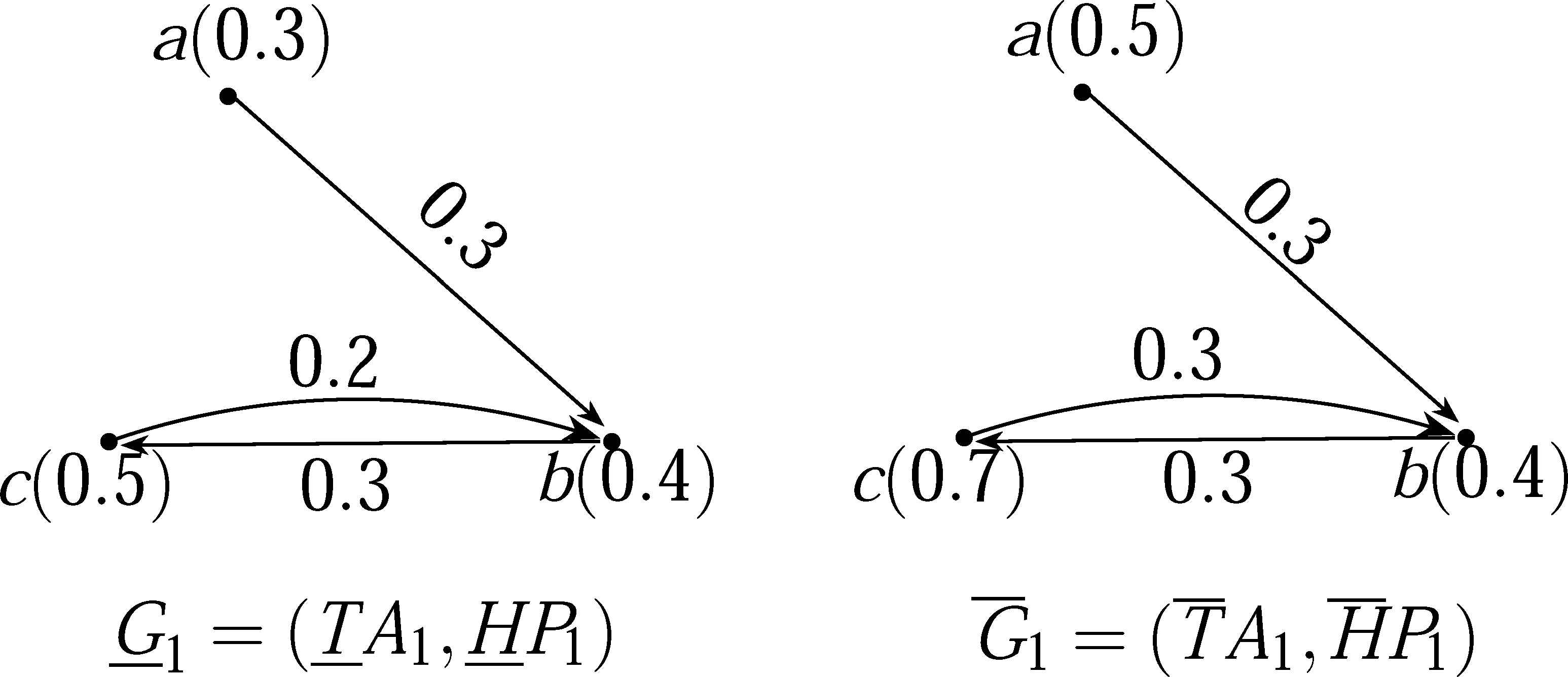
Lower and upper approximations of G2
The composition of G1 and G2 is
Lower and upper approximations of G1 ◦G2
Theorem 3.
Let
Proof.
By using similar arguments as used in the proof of Theorem 2.3 of 4, the proof is straightforward.
Definition 10.
Let
- (i)
- (ii)
Example 7.
consider a fuzzy rough digraph G as shown in Fig. 10.
Lower and upper approximations of G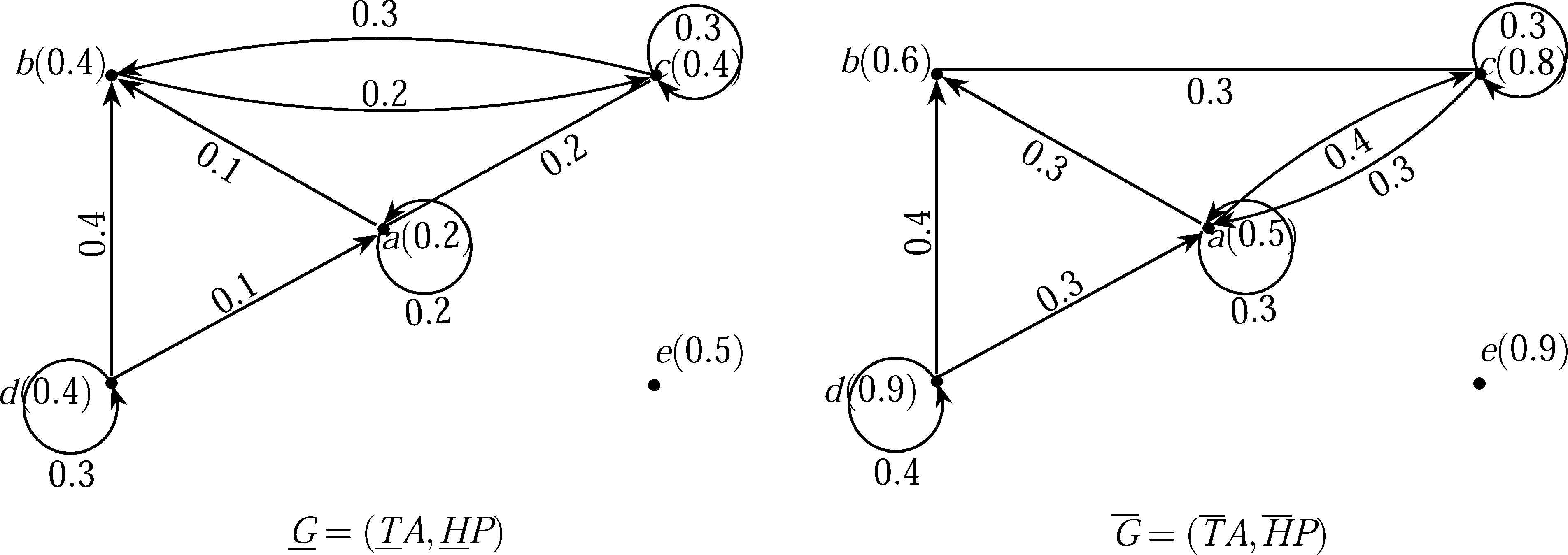
The complement of G is
Lower and upper approximations of Gc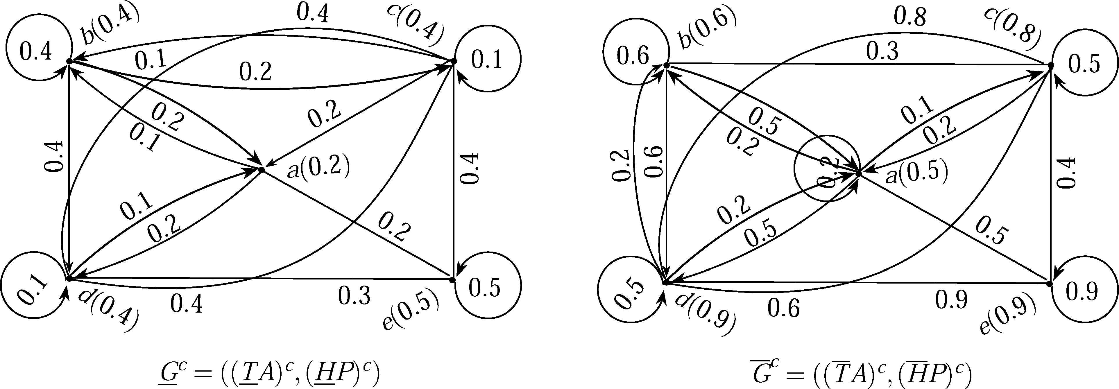
Definition 11.
A fuzzy rough digraph is self complementary if G and Gc are isomorphic, i.e.,
Example 8.
Let U = {a,b,c,d} be a set. and T a fuzzy tolerance relation on U defined as in Table 3. Let A = {(a,0.8),(b,0.6),(c,0.4),(d,0.6)} be a fuzzy set on U and
| T | a | b | c | d |
|---|---|---|---|---|
| a | 1 | 0.6 | 0.4 | 0.8 |
| b | 0.6 | 1 | 0.6 | 0.8 |
| c | 0.4 | 0.6 | 1 | 0.4 |
| d | 0.8 | 0.8 | 0.4 | 1 |
Fuzzy tolerance relation T
Let P* = {aa, ab, ac, ad, ba, bb, bc, bd, ca, cb, cc, cd, da, db, dc, dd} ⊆ U × U and H a fuzzy tolerance relation on P* defined as in Table 4. Let P = {(aa,0.4), (ab,0.3), (ac,0.3), (ad,0.3), (ba,0.3), (bb,0.2), (bc,0.2), (bd,0.2), (ca,0.2), (cb,0.3), (cc,0.2), (cd,0.2), (da,0.3), (db,0.2), (dc,0.2), (dd,0.4)} be a fuzzy set on P* and
| H | aa | ab | ac | ad | ba | bb | bc | bd | ca | cb | cc | cd | da | db | dc | dd |
|---|---|---|---|---|---|---|---|---|---|---|---|---|---|---|---|---|
| aa | 1 | 0.3 | 0.3 | 0.7 | 0.3 | 0.3 | 0.3 | 0.2 | 0.3 | 0.2 | 0.2 | 0.3 | 0.4 | 0.3 | 0.2 | 0.6 |
| ab | 0.3 | 1 | 0.3 | 0.8 | 0.3 | 0.6 | 0.4 | 0.4 | 0.4 | 0.3 | 0.4 | 0.2 | 0.2 | 0.8 | 0.6 | 0.3 |
| ac | 0.3 | 0.3 | 1 | 0.4 | 0.3 | 0.4 | 0.4 | 0.4 | 0.2 | 0.2 | 0.4 | 0.2 | 0.3 | 0.2 | 0.8 | 0.2 |
| ad | 0.7 | 0.8 | 0.4 | 1 | 0.6 | 0.6 | 0.4 | 0.4 | 0.4 | 0.2 | 0.4 | 0.4 | 0.4 | 0.4 | 0.4 | 0.7 |
| ba | 0.3 | 0.3 | 0.3 | 0.6 | 1 | 0.6 | 0.4 | 0.8 | 0.6 | 0.3 | 0.4 | 0.4 | 0.3 | 0.6 | 0.4 | 0.3 |
| bb | 0.3 | 0.6 | 0.4 | 0.6 | 0.6 | 1 | 0.6 | 0.8 | 0.4 | 0.3 | 0.4 | 0.6 | 0.3 | 0.6 | 0.6 | 0.3 |
| bc | 0.3 | 0.4 | 0.4 | 0.4 | 0.4 | 0.6 | 1 | 0.4 | 0.4 | 0.3 | 0.6 | 0.4 | 0.2 | 0.4 | 0.8 | 0.3 |
| bd | 0.2 | 0.4 | 0.4 | 0.4 | 0.8 | 0.8 | 0.4 | 1 | 0.6 | 0.3 | 0.2 | 0.4 | 0.3 | 0.6 | 0.4 | 0.3 |
| ca | 0.3 | 0.4 | 0.2 | 0.4 | 0.6 | 0.4 | 0.4 | 0.6 | 1 | 0.3 | 0.4 | 0.8 | 0.3 | 0.4 | 0.4 | 0.3 |
| cb | 0.2 | 0.3 | 0.2 | 0.2 | 0.3 | 0.3 | 0.3 | 0.3 | 0.3 | 1 | 0.4 | 0.8 | 0.3 | 0.2 | 0.4 | 0.3 |
| cc | 0.2 | 0.4 | 0.4 | 0.4 | 0.4 | 0.4 | 0.6 | 0.2 | 0.4 | 0.4 | 1 | 0.4 | 0.2 | 0.4 | 0.4 | 0.3 |
| cd | 0.3 | 0.2 | 0.2 | 0.4 | 0.4 | 0.6 | 0.4 | 0.4 | 0.8 | 0.8 | 0.4 | 1 | 0.3 | 0.4 | 0.2 | 0.3 |
| da | 0.4 | 0.2 | 0.3 | 0.4 | 0.3 | 0.3 | 0.2 | 0.3 | 0.3 | 0.3 | 0.2 | 0.3 | 1 | 0.3 | 0.4 | 0.7 |
| db | 0.3 | 0.8 | 0.2 | 0.4 | 0.6 | 0.6 | 0.4 | 0.6 | 0.4 | 0.2 | 0.4 | 0.4 | 0.3 | 1 | 0.4 | 0.3 |
| dc | 0.2 | 0.6 | 0.8 | 0.4 | 0.4 | 0.6 | 0.8 | 0.4 | 0.4 | 0.4 | 0.4 | 0.2 | 0.4 | 0.4 | 1 | 0.3 |
| dd | 0.6 | 0.3 | 0.2 | 0.7 | 0.3 | 0.3 | 0.3 | 0.3 | 0.3 | 0.3 | 0.3 | 0.3 | 0.7 | 0.3 | 0.3 | 1 |
Fuzzy tolerance relation H
Thus,
Lower and upper approximations of Gc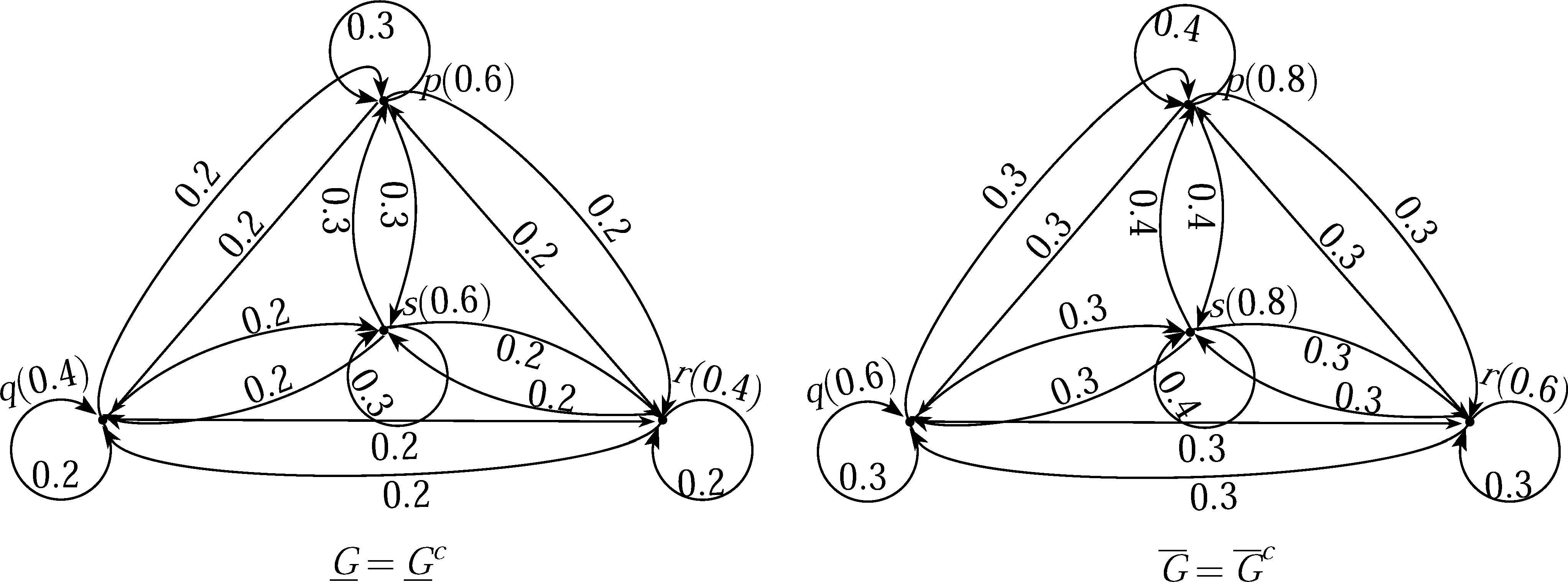
The complement of G is
Theorem 4.
Let
Proof.
By using similar arguments as used in the proof of Theorem 2.4 of 4, the proof is straightforward.
Theorem 5.
Let
Then G is self complementary.
Proof.
By using similar arguments as used in the proof of Theorem 2.5 of 4, the proof is straightforward.
Definition 12.
Let
- (i)
- (ii)
Example 9.
Let U = {a,b,c} be a set. Let
Lower and upper approximations of G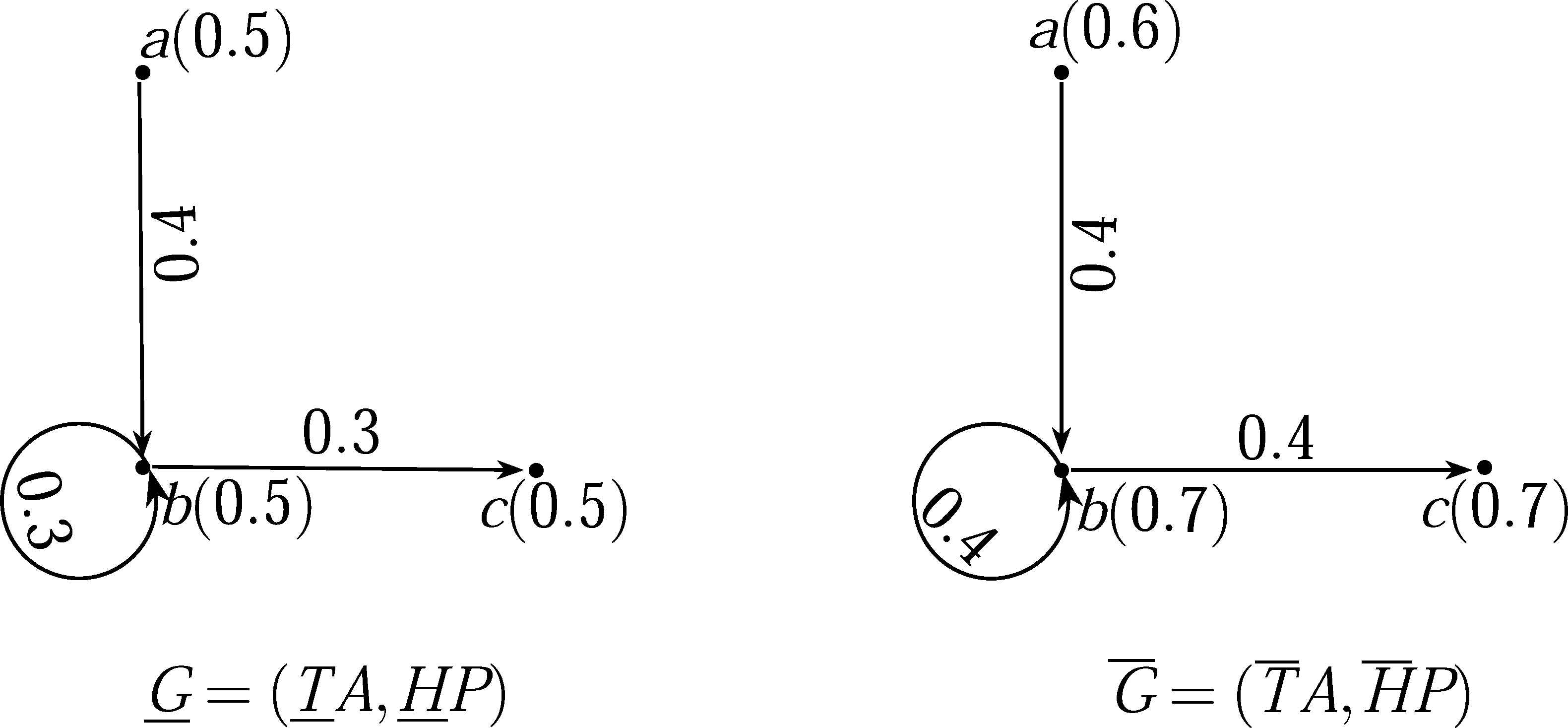
The μ − complement of G is
Lower and upper approximations of Gμ
Definition 13.
A fuzzy rough digraph is self μ − complementary if G and Gμ are isomorphic, i.e.,
Example 10.
Let U = {a,b,c,d} be a set. and T a fuzzy tolerance relation on U defined as in Table 5.
| T | a | b | c | d |
|---|---|---|---|---|
| a | 1 | 0.6 | 0.8 | 0.4 |
| b | 0.6 | 1 | 0.4 | 0.6 |
| c | 0.8 | 0.4 | 1 | 0.8 |
| d | 0.4 | 0.6 | 0.8 | 1 |
Fuzzy tolerance relation T
Let A = {(a,0.7),(b,0.6),(c,0.8),(d,0.4)} be a fuzzy set on U and
Let P* = { aa, ab, bb, ac, ca, bd, db} ⊆ U × U and H a fuzzy tolerance relation on P* defined as in Table 6.
| H | aa | ab | bb | bc | cc | cd | dd | da | ac | ca | bd | db |
|---|---|---|---|---|---|---|---|---|---|---|---|---|
| aa | 1 | 0.3 | 0.3 | 0.3 | 0.6 | 0.4 | 0.4 | 0.3 | 0.7 | 0.7 | 0.3 | 0.3 |
| ab | 0.3 | 1 | 0.4 | 0.4 | 0.3 | 0.4 | 0.2 | 0.2 | 0.4 | 0.4 | 0.5 | 0.2 |
| bb | 0.3 | 0.4 | 1 | 0.2 | 0.3 | 0.4 | 0.4 | 0.6 | 0.4 | 0.4 | 0.6 | 0.6 |
| bc | 0.3 | 0.4 | 0.2 | 1 | 0.3 | 0.4 | 0.6 | 0.5 | 0.4 | 0.7 | 0.8 | 0.4 |
| cc | 0.6 | 0.3 | 0.3 | 0.3 | 1 | 0.3 | 0.5 | 0.6 | 0.8 | 0.4 | 0.3 | 0.2 |
| cd | 0.4 | 0.4 | 0.4 | 0.4 | 0.3 | 1 | 0.8 | 0.3 | 0.6 | 0.4 | 0.4 | 0.4 |
| dd | 0.2 | 0.2 | 0.5 | 0.6 | 0.5 | 0.8 | 1 | 0.3 | 0.4 | 0.4 | 0.4 | 0.4 |
| da | 0.3 | 0.2 | 0.6 | 0.5 | 0.6 | 0.3 | 0.3 | 1 | 0.4 | 0.8 | 0.4 | 0.4 |
| ac | 0.7 | 0.4 | 0.4 | 0.4 | 0.8 | 0.6 | 0.4 | 0.4 | 1 | 0.8 | 0.6 | 0.2 |
| ca | 0.7 | 0.4 | 0.4 | 0.7 | 0.4 | 0.4 | 0.4 | 0.8 | 0.8 | 1 | 0.3 | 0.4 |
| bd | 0.3 | 0.5 | 0.6 | 0.8 | 0.3 | 0.4 | 0.4 | 0.4 | 0.6 | 0.3 | 1 | 0.4 |
| db | 0.3 | 0.2 | 0.6 | 0.4 | 0.2 | 0.4 | 0.4 | 0.4 | 0.2 | 0.4 | 0.4 | 1 |
Fuzzy tolerance relation H
Let P = { (aa,0.4), (ab,0.2), (bb,0.2), (bc,0.3), (cc,0.4), (cd,0.2), (dd,0.3), (da,0.2), (ac,0.2), (ca,0.3), (bd,0.2), (db,0.2)} be a fuzzy set on P* and
Thus,
Lower and upper approximations of Gμ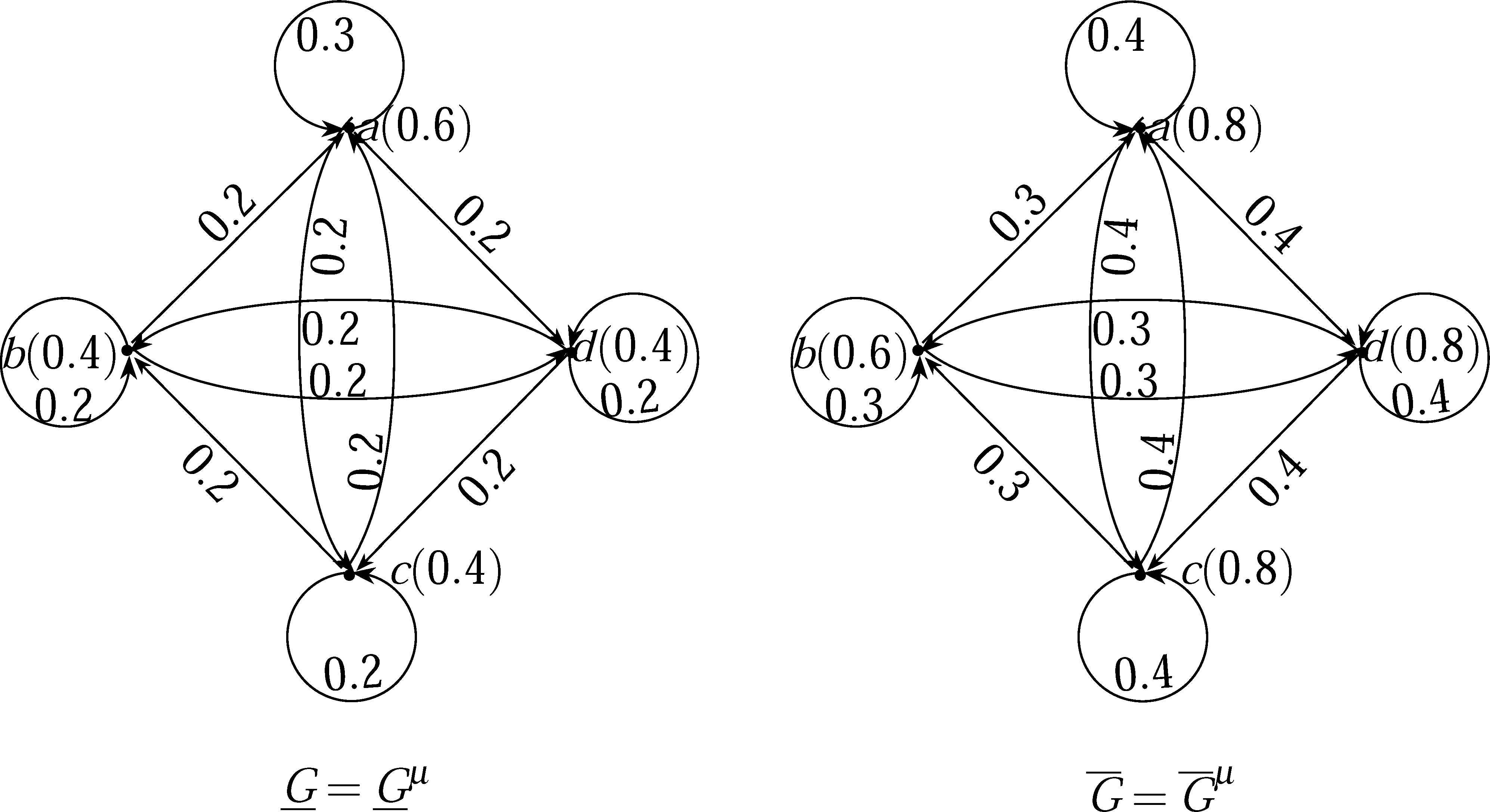
The μ − complement of G is
We state the following results without their proofs.
Theorem 6.
Let
Theorem 7.
Let
Then G is self μ − complementary.
3. Applications
Decision making is very important in our daily life. There are many uncertain systems and decision making under uncertainty or the choice in uncertain environment is the central subject in many of the disciplines that are alloyed in management curriculum. Decision making is the process of identifying a problem, developing alternatives, evaluating all possible alternatives and then selecting the best one. In this section, we present an approach to decision-making under uncertain systems using fuzzy rough information. This method gives deep considerations of the problem as it involves lower and upper approximations of the given uncertain information.
3.1. Selection of a city for treatment
Emerging infectious diseases can be defined as infections that have newly appeared in a population or have existed but are rapidly increasing in incidence or geographic range. Among recent examples are Dengue fever and respiratory disease. Some infectious diseases are transmitted by bites of insects or animals and others are acquired by ingesting contaminated food. But some precautions are there that can be done to prevent from these diseases.
Consider an example of a manager of health care organization who wants to prevent the society from these infectious diseases. He has a number of cities under consideration. He collected information about emerging infectious diseases in different cities and causes of them. After investigation, he concluded that human population density is a key factor for the emergence of infectious diseases. He has a problem to choose one city that should be treated first. He will select that city which will have the maximum choice value among others. The problem can be represented by a fuzzy rough digraph whose vertices represent the cities and there is an edge between them if the areas joining them have increasing population density. Consider a network of eight cities U = {C1,C2,C3,C4,C5,C6,C7,C8}. Let T be fuzzy tolerance relation on U defined as in Table 7.
| T | C1 | C2 | C3 | C4 | C5 | C6 | C7 | C8 |
|---|---|---|---|---|---|---|---|---|
| C1 | 1 | 0.7 | 0.8 | 0.9 | 0.6 | 0.5 | 0.7 | 0.6 |
| C2 | 0.7 | 1 | 0.4 | 0.3 | 0.5 | 0.9 | 0.8 | 0.2 |
| C3 | 0.8 | 0.4 | 1 | 0.5 | 0.7 | 0.6 | 0.3 | 0.4 |
| C4 | 0.9 | 0.3 | 0.5 | 1 | 0.4 | 0.8 | 0.9 | 0.7 |
| C5 | 0.6 | 0.5 | 0.7 | 0.4 | 1 | 0.6 | 0.5 | 0.8 |
| C6 | 0.5 | 0.9 | 0.6 | 0.8 | 0.6 | 1 | 0.4 | 0.3 |
| C7 | 0.7 | 0.8 | 0.3 | 0.9 | 0.5 | 0.4 | 1 | 0.9 |
| C8 | 0.6 | 0.2 | 0.4 | 0.7 | 0.8 | 0.3 | 0.9 | 1 |
Fuzzy tolerance relation T
where T(Ci,Cj) represents the relationship of comparison between degree of emerging infectious diseases in Ci and degree of emerging infectious diseases in Cj. Let A = { (C1,0.7), (C2,0.9), (C3,0.6), (C4,0.5), (C5,0.6), (C6,0.7), (C7,0.8), (C8,0.9)} be a fuzzy set on U describing the degree of emerging infectious diseases in each city and
Let P* = { C1C2, C1C3, C2C4, C3C2, C3C5, C3C7, C4C6, C4C7, C5C7, C6C2, C7C8, C8C6} ⊆ U × U.
Let P = { (C1C2,0.45), (C1C3,0.4), (C2C4,0.39), (C3C2,0.42), (C3C5,0.47), (C3C7,0.35), (C4C6,0.46), (C4C7,0.38), (C5C7,0.45), (C6C2,0.49), (C7C8,0.43), (C8C6,0.37)} be a fuzzy set on P* where P(Ci,Cj) (i, j = 1,2,…,8) represents the degree of increase in population density when we travel from Ci towards Cj and let H be fuzzy tolerance relation on P* defined as in Table 8. where H(CiCj,CkCl) Ci,Cj ∈ P* represents the relationship of comparison between P(CiCj) and P(CiCj). The set
| H | C1 | C1 | C2 | C3 | C3 | C3 | C4 | C4 | C5 | C6 | C7 | C8 |
|---|---|---|---|---|---|---|---|---|---|---|---|---|
| C2 | C3 | C4 | C2 | C5 | C7 | C6 | C7 | C7 | C2 | C8 | C6 | |
| C1C2 | 1 | 0.3 | 0.3 | 0.7 | 0.4 | 0.7 | 0.8 | 0.6 | 0.5 | 0.4 | 0.2 | 0.5 |
| C1C3 | 0.3 | 1 | 0.4 | 0.3 | 0.6 | 0.2 | 0.5 | 0.2 | 0.2 | 0.3 | 0.3 | 0.5 |
| C2C4 | 0.3 | 0.4 | 1 | 0.3 | 0.3 | 0.4 | 0.2 | 0.2 | 0.5 | 0.2 | 0.6 | 0.2 |
| C3C2 | 0.7 | 0.3 | 0.3 | 1 | 0.4 | 0.7 | 0.5 | 0.4 | 0.6 | 0.5 | 0.2 | 0.3 |
| C3C5 | 0.4 | 0.6 | 0.3 | 0.4 | 1 | 0.4 | 0.4 | 0.5 | 0.4 | 0.4 | 0.2 | 0.3 |
| C3C7 | 0.7 | 0.2 | 0.4 | 0.7 | 0.4 | 1 | 0.3 | 0.4 | 0.6 | 0.5 | 0.2 | 0.4 |
| C4C6 | 0.8 | 0.5 | 0.2 | 0.5 | 0.4 | 0.3 | 1 | 0.3 | 0.3 | 0.7 | 0.2 | 0.6 |
| C4C7 | 0.6 | 0.2 | 0.2 | 0.4 | 0.5 | 0.4 | 0.3 | 1 | 0.3 | 0.6 | 0.8 | 0.3 |
| C5C7 | 0.5 | 0.2 | 0.5 | 0.6 | 0.4 | 0.6 | 0.3 | 0.3 | 1 | 0.5 | 0.4 | 0.3 |
| C6C2 | 0.4 | 0.3 | 0.2 | 0.5 | 0.4 | 0.5 | 0.7 | 0.6 | 0.5 | 1 | 0.2 | 0.2 |
| C7C8 | 0.2 | 0.3 | 0.6 | 0.2 | 0.2 | 0.2 | 0.2 | 0.8 | 0.4 | 0.2 | 1 | 0.3 |
| C8C6 | 0.5 | 0.5 | 0.2 | 0.3 | 0.3 | 0.4 | 0.6 | 0.3 | 0.3 | 0.2 | 0.3 | 1 |
Fuzzy tolerance relation H
By using this fuzzy rough information, fuzzy rough digraph can be drawn as shown in Fig. 16. To identify the required city, here is required to determine a vertex which will have maximum choice value among others.
Lower and upper approximations of G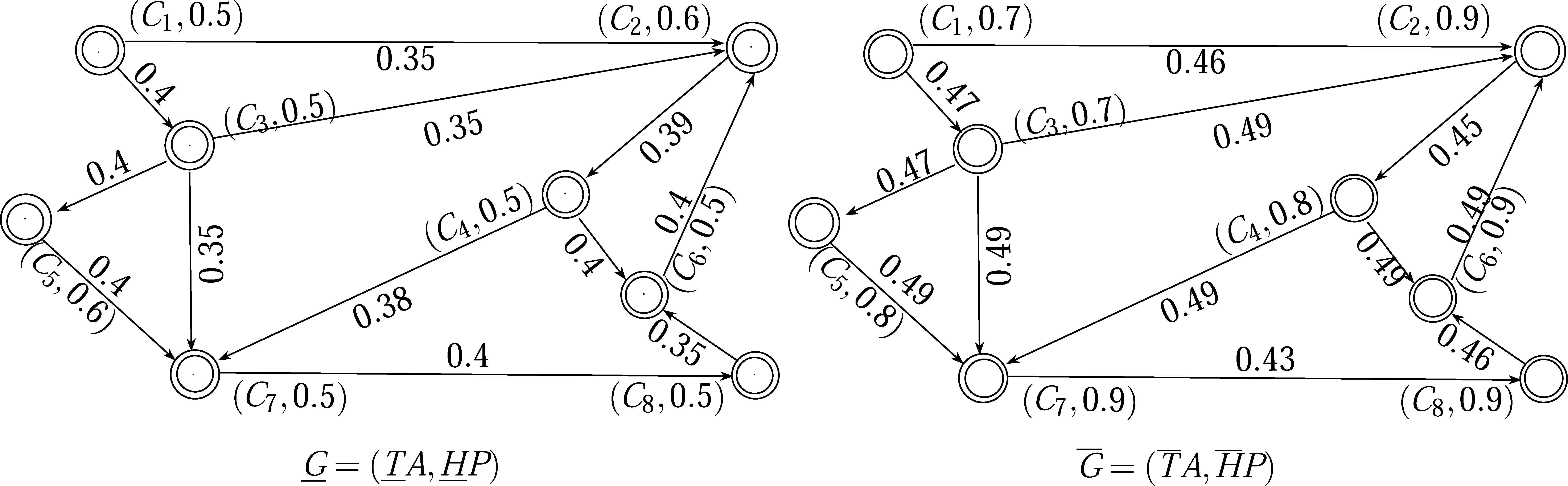
By using formula,
Hence, C7 is the most effected city and should be treated first.
The algorithm for determining a vertex with maximum choice value is shown in Table 9. The net time complexity of the algorithm is either O(n2r) if n2 r > r2 or O(r2) if n2 r < r2 where, n is the number of vertices and r is the number of edges.
| Algorithm for rough fuzzy digraph |
|---|
Begin
|
Determining a vertex with maximum choice value
3.2. Identification of best location in a department to set mobile phone Jammer
Consider an example of an institute whose director wants to set up mobile phone jammer in a number of departments in such a way that every department is in the effect of at least one of the jammer. To reduce the cost to set up strong and high quality jammer, it is required to set up minimum number of jammer. Consider a network of seven departments U = {D1, D2, D3, D4, D5, D6, D7}.
Let T be fuzzy tolerance relation on U defined as in Table 10. Where T(Di,Dj), (i, j = 1,2,…,7) represents the relationship of comparison between strength of jammer in Di and strength of jammer in Dj.
| T | D1 | D2 | D3 | D4 | D5 | D6 | D7 |
|---|---|---|---|---|---|---|---|
| D1 | 1 | 0.4 | 0.5 | 0.5 | 0.3 | 0.5 | 0.6 |
| D2 | 0.4 | 1 | 0.4 | 0.5 | 0.6 | 0.6 | 0.6 |
| D3 | 0.5 | 0.4 | 1 | 0.7 | 0.6 | 0.6 | 0.5 |
| D4 | 0.5 | 0.5 | 0.7 | 1 | 0.4 | 0.6 | 0.6 |
| D5 | 0.3 | 0.6 | 0.6 | 0.4 | 1 | 0.9 | 0.2 |
| D6 | 0.5 | 0.6 | 0.6 | 0.6 | 0.9 | 1 | 0.6 |
| D7 | 0.6 | 0.6 | 0.5 | 0.6 | 0.2 | 0.6 | 1 |
Fuzzy tolerance relation T
Let A = {(D1,0.5), (D2,0.7), (D3,0.6), (D4,0.6), (D5,0.6), (D6,0.6), (D7,0.6)} be a fuzzy set on U which describes the strength of jammer in each department and
Let P* = {D2D1, D3D2, D3D1, D3D4, D3D6, D4D1, D5D3, D5D6, D5D7, D6D7} ⊆ U × U.
Let H be fuzzy tolerance relation on P* defined as in Table 11. H(DiDj,DkDl) DiDj,DkDl ∈P* describes the relationship of comparison between P(DiDj) and P(DkDl) where P = { (D2D1,0.5), (D3D2,0.5), (D3D1,0.5), (D3D4,0.5), (D3D6,0.5), (D4D1,0.5), (D5D3,0.4), (D5D6,0.5), (D5D7,0.6), (D6D7,0.5)} is fuzzy set on P* and P(DiDj) DiDj ∈ P* describes the degree of interference created by jammers of Di at the same frequency range that is used by cell phones in the surroundings of Dj. The set
| H | D2 | D3 | D3 | D3 | D3 | D4 | D5 | D5 | D5 | D6 |
|---|---|---|---|---|---|---|---|---|---|---|
| D1 | D2 | D1 | D4 | D6 | D1 | D3 | D6 | D7 | D7 | |
| D2D1 | 1 | 0.3 | 0.3 | 0.4 | 0.4 | 0.5 | 0.5 | 0.4 | 0.2 | 0.2 |
| D3D2 | 0.3 | 1 | 0.3 | 0.4 | 0.5 | 0.3 | 0.4 | 0.5 | 0.6 | 0.3 |
| D3D1 | 0.3 | 0.3 | 1 | 0.5 | 0.5 | 0.6 | 0.5 | 0.5 | 0.6 | 0.2 |
| D3D4 | 0.4 | 0.4 | 0.5 | 1 | 0.5 | 0.5 | 0.4 | 0.5 | 0.6 | 0.3 |
| D3D6 | 0.4 | 0.5 | 0.5 | 0.5 | 1 | 0.5 | 0.6 | 0.5 | 0.2 | 0.2 |
| D4D1 | 0.5 | 0.3 | 0.6 | 0.5 | 0.5 | 1 | 0.3 | 0.3 | 0.2 | 0.2 |
| D5D3 | 0.5 | 0.4 | 0.5 | 0.4 | 0.6 | 0.3 | 1 | 0.5 | 0.4 | 0.4 |
| D5D6 | 0.4 | 0.5 | 0.5 | 0.5 | 0.5 | 0.3 | 0.5 | 1 | 0.6 | 0.2 |
| D5D7 | 0.2 | 0.6 | 0.6 | 0.6 | 0.2 | 0.2 | 0.4 | 0.6 | 1 | 0.4 |
| D6D7 | 0.2 | 0.3 | 0.2 | 0.3 | 0.2 | 0.2 | 0.4 | 0.2 | 0.4 | 1 |
Fuzzy tolerance relation H
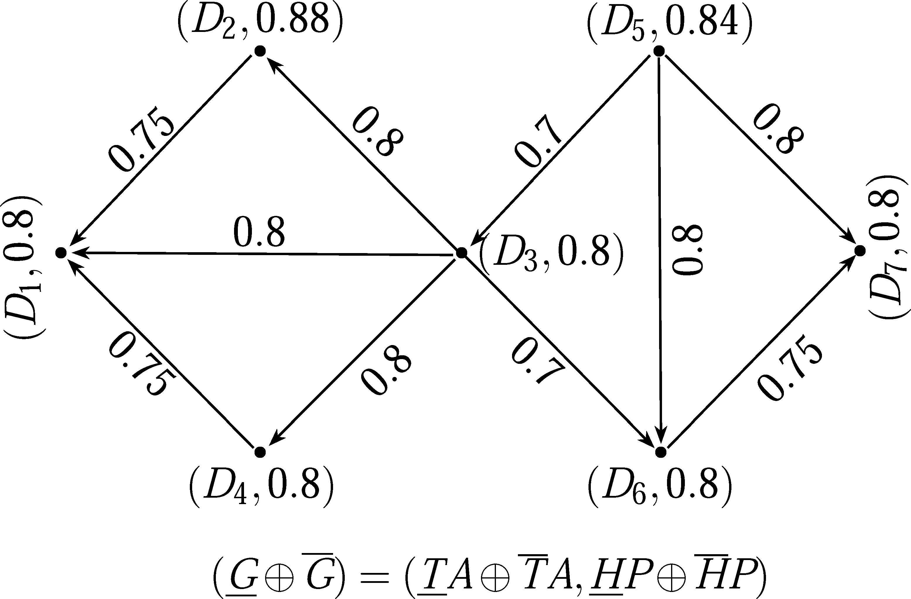
The problem can be represented by fuzzy rough digraphs as shown in Fig. 17. where vertices represent the departments and there is an edge between vertices, if one is in the effect of the gammer set up in the other. Applying the following formulae.

Lower and upper approximations of G
It implies that,
Hence we have a fuzzy digraph as shown in Fig. 18.
Fuzzy digraph
The final step is to just determine the minimal dominating set of the above digraph which will be the required solution. The dominating set is {D3,D5}. Hence by setting jammer only in D3 and D5, it can be reduced the cost.
The method of calculating a minimal dominating set is described as an algorithm in Table 12.
| Algorithm |
|---|
|
Algorithm for determining a minimal dominating set
4. A View of Fuzzy Rough Graphs in Comparison with Fuzzy Graphs
The concept of fuzzy set has been utilized successfully to model uncertainty in different domains of science and technology. Due to the limitation of human knowledge to understand complex problems, it is difficult to apply single type of uncertain methods to deal with real life problems. In decision-making problems, it is required to consider parametric uncertainty in graphical models. For example, in the selection of a best organization for social work, we are not only interested in analyzing the working rules and characteristics of these organizations but also the evaluation of co-ordination relation between each pair of alternatives. Fuzzy rough set theory is a novel mathematical tool to overcome this difficulty. It provides lower and upper approximation of target set using fuzzy tolerance relation between any two objects. Here we present the numerical comparison of fuzzy rough graphs with fuzzy graphs by applying fuzzy sets to above described application as follows: The problem described in subsection 3.2, can be represented using fuzzy digraphs as follows.
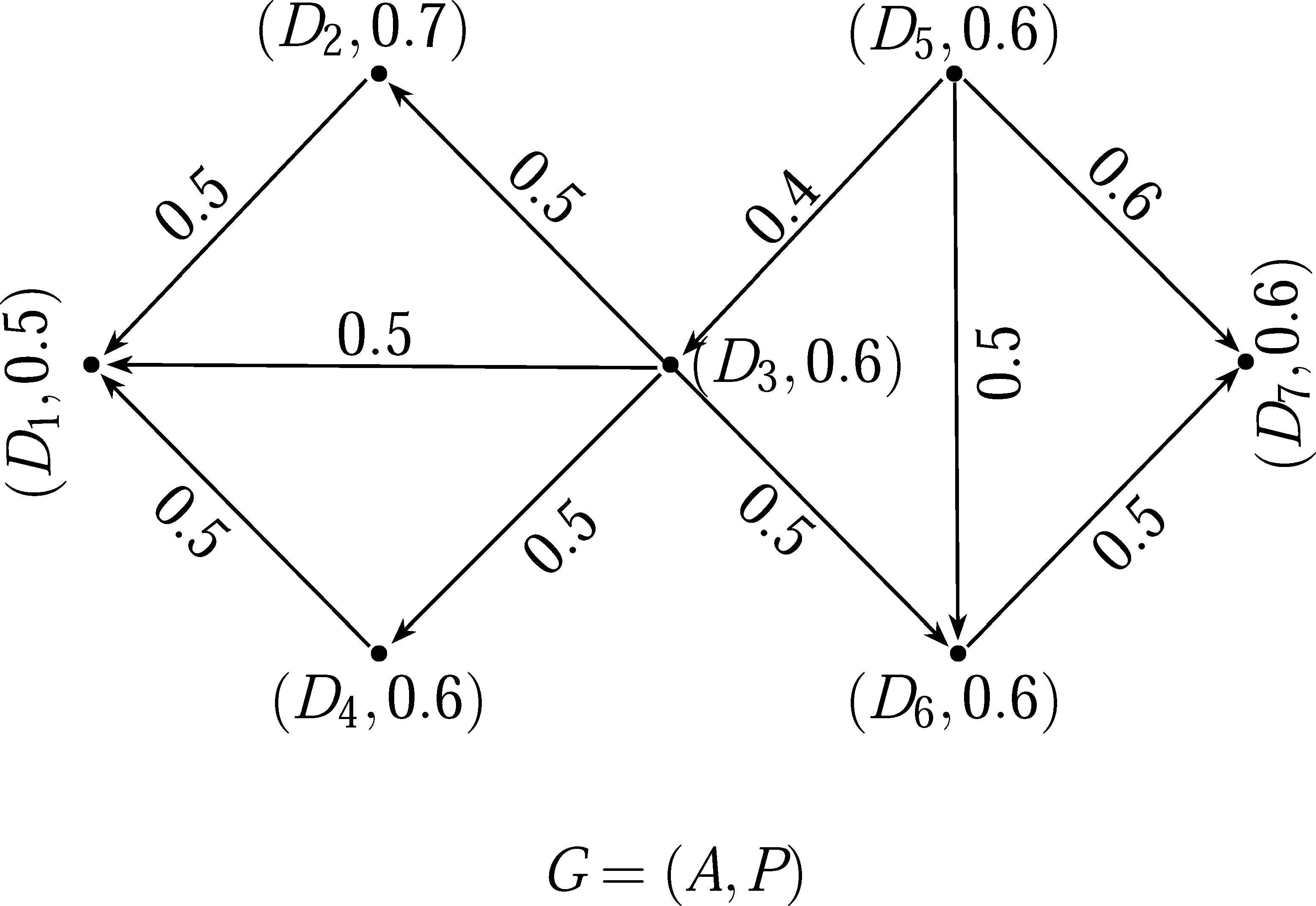
Fuzzy digraph G = (A,P)
5. Conclusions
Fuzzy rough set theory gives the upper and lower approximations of a fuzzy set. In existing literature, an arbitrary and equivalence relation have been used as approximation tools in generalized rough set theory and Pawlak rough set theory, respectively. In this paper, we have developed a method using fuzzy tolerance relation as an approximation tool. We have introduced the notions of fuzzy rough relations and fuzzy rough digraphs. Fuzzy rough digraphs can be viewed as upper and lower approximation of fuzzy digraphs. We have presented fuzzy rough digraphs as an enormous tool to solve uncertain decision-making problems.
Acknowledgements:
The authors are very thankful to an Associate Editor and referees for their valuable comments and suggestions for improving the paper.
References
Cite this article
TY  - JOUR
AU  - Muhammad Akram
AU  - Maham Arshad
AU  - Shumaiza
PY  - 2018
DA  - 2018/11/01
TI  - Fuzzy Rough Graph Theory with Applications
JO  - International Journal of Computational Intelligence Systems
SP  - 90
EP  - 107
VL  - 12
IS  - 1
SN  - 1875-6883
UR  - https://doi.org/10.2991/ijcis.2018.25905184
DO  - 10.2991/ijcis.2018.25905184
ID  - Akram2018
ER  -