2.1. Hadoop Parameters

The most important and fundamental concept of Hadoop is to reduce the overall processing time by distributing one task to multiple cluster nodes. To control the efficient operation between master and slave nodes [13], tuning of configuration parameter according to system environment is needed. Well-tuned parameter values will keep the system in optimal condition and ultimately improve system performance.

Apache Hadoop has more than 80 parameters [14] and 25 of these parameters are significantly affected map and reduce performance [4]. Those parameters are defined at the $hadoop_home/conf/mapred-site.xml as one of the properties. For example, io.sort.mb with default value 100 and io.sort.record.percent with value 0.05 can be described as follows:

• •

  Configuration for mapred-site.xml

  <configuration>

  <property>

  <name>io.sort.mb</name>

  <value>100</value>

  </property>

  <property>

  <name>io.sort.record.percent</name>

  <value>0.05</value>

  </property>

  <property>

  <name>io.sort.spill.percent</name>

  <value>0.80</value>

  </property>

  <property>

  <name>io.sort.factor</name>

  <value>10</value>

  </property>

  <property>

  <name>mapred.job.shuffle.merge.percent

  </name>

  <value>0.66</value>

  </property>

  <property>

  <name>mapred.job.shuffle.input.buffer.percent</name>

  <value>0.70</value>

  </property>

  </configuration>

There are several steps to set up parameter values static way, first stop all the processes (Hadoop SecondaryNameNode, DataNode, TaskTracker, JobTracker, NameNode) on the cluster using stop-all.sh, manually modify the configuration, and then use start-all.sh to start all the processes. Apache Hadoop operates using the default value defined in $hadoop_home/docs/hdfs-default.xml, if required parameters are not defined in the $hadoop_home/conf/mapred-site.xml.

At the previous work we have developed a java application framework to modify configuration files without human intervention and applied at the several parameter evaluations [9–12].

As shown in Table 1, we have selected six important parameters for evaluation set which includes a domain of double or integer type. Each parameter distinguishes the minimum value from the maximum value based on the default value. When the tuning is completed, one value will be determined for each parameter.

2.2. Parameter Value Domains

As shown in Table 2, all parameter values are constantly subdivided by ranging from −90% up to +90% based on its low and high values [11]. The reason for configuring this arity table is to broaden the selection that one parameter can have.

2.3. Parameter Space

The parameter space [9,11], denoted by Ω(x) is a sample space composed of parameter combinations taken from arity table and its time difference generated by map and reduce applications.

Depending on the algorithm chosen, the number of parameter combinations can be variably changed. If we apply Naïve exhaustive algorithm, the size of the space will hold a^p cases with its evaluation results (where a: arity, n: number of parameter).

While the heuristically greedy algorithm requires multiple Ω(x) spaces which will hold each cases respectively, e.g., a * p, a * (p − 1), a * (p − 2), …, a * (p − (p − 1)).

2.4. Benchmarking Applications

Apache Hadoop distribution provide predeveloped several stress testing tools such as TestDFSIO, TeraSort, MrBench and MnBench in forms of hadoop-test-1.2.1.jar or hadoop-examples-1.2.1.jar.

The TestDFSIO [12] for measuring throughput, average IO rate mb/s, IO rate std deviation, and execution time on the HDFS clusters are as follows:

• (e.g. -nrFiles 10, -fileSize 100)

  ----- TestDFSIO -----: write

  Date & time: Fri Oct 19 21:38:29 EDT 2018

  Number of files: 10

  Total MBytes processed: 1000

  Throughput mb/s: 1.6357509732718292

  Average IO rate mb/s: 1.6582612991333008

  IO rate std deviation: 0.2057749407824309

  Test exec time sec: 82.103

  ----- TestDFSIO -----: read

  Date & time: Fri Oct 19 21:44:03 EDT 2018

  Number of files: 10

  Total MBytes processed: 905

  Throughput mb/s: 6.272530530132189

  Average IO rate mb/s: 35.75289535522461

  IO rate std deviation: 88.22740064015464

  Test exec time sec: 40.019

The TeraSort [12] is a benchmark that combines testing the HDFS and MapReduce of a Hadoop cluster [15]. It provides MapReduce framework, File system counters, and Job Counters.

The MrBench [12] is an application to measure performance by executing several small-scale jobs multiple times, as opposed to large tasks on TeraSort. Following example shows average time consumption for 30 runs.

$ hadoop jar hadoop-*test*.jar mrbench -numRuns 30

2.5. Cost of the Parameter Selection Algorithms

The execution time of map and reduce task will not be estimated before evaluation process has finished. This is because the correlation between one value of parameter and the others does not have a linear relationship. To verify this, we have to create a combination of values and run each case in the actual Hadoop environment. If it takes too much time, benchmarking will be less effective.

Considering three methods we have proposed, we can express the execution time as a Big O notation as follows:

2.5.1 Cost comparison

• > Naïve exhaustive: O(a^p)

• > Random method: O(1 * p * r) ≈ O(P^2)

• > Greedy: O(a*(p + (p − 1) + (p − 2) + … p − (p − 1))) ≈ O (p^3)

Where, p: number of parameters, 1: constant time, a: number of parameter values.

The execution time of Naïve exhaustive method can be expressed as O(a^p) because you have to take into account the number of all cases, which in other words can be called the combinatorial problem. This approach is beneficial for finding appropriate parameters, but there is a time-consuming disadvantage.

To compensate for these drawbacks, the random method proposed. In this method, a parameter value is picked from the arity table by generating random numbers ranging from zero to 17. With this method, we could shorten the execution time, but we could not find a good candidate parameter compared to the Naïve exhaustive.

Finally, the heuristically greedy proposed to save benchmarking time and find acceptable parameters. An important point of this method was to fix the parameter value that most drastically reduced execution time in one parameter space and to test other parameters based on it.

Figure 1 shows how the benchmarking time changes as the number of parameters to be tested increases. Here we can see the heuristically greedy lies between Naïve and Random, but almost similar to Random’s execution time.

Figure 1

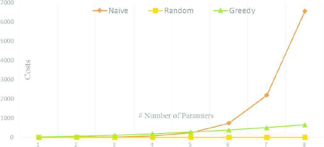
Optimization cost of e-Heuristic greedy

It is difficult to determine a linear correlation between each parameter combination.

The heuristically greedy method is less efficient compared to the random [10], but it has been verified in previous studies as a computationally feasible way to find the best combination of parameters. The heuristically-based parametric optimization took slightly over quadratic time or at most cubic time and the performance is also great with feasible optimization time [11].

3.1. e-Heuristic Greedy Structure and Operations

The overall main logic of e-Heuristic greedy is similar to heuristically greedy, but in the e-heuristic greedy, two more functions are combined to hold MrBench and TestDFSIO benchmarks. This model takes the form of batch processing. Once it is executed, the Hadoop configuration is created and three benchmarking programs are sequentially executed based on this configuration. This is because Hadoop HDFS must be restarted to apply changed parameter values for the new task. The component of the parameter space that we set conceptually defined are stored in a single text file in the Linux system.

3.2. e-Heuristic Greedy – Parameter Space

The parameter evaluation space denoted by Ω composed of n − 1 spaces from Ω(0), Ω(1), …, Ω(n − 1) where n: number of configuration parameters. The Ω(0) is an initial evaluation space for all parameters which includes set of values of parameter and its evaluation results generated by benchmarking applications.

The first benchmarking uses the default parameter values (i.s.m 100, i.s.r.p 0.05, i.s.s.p 0.80, i.s.f 10, m.j.s.m.p 0.66, m.j.s.i.b.p 0.70) provided by Hadoop distribution. Based on this subsequent processing continues with this value and the result is stored in the Ω(x + 1).

As shown in Table 3, the Ω(x) space is composed of parameter values taken from the arity table and the execution time difference value of benchmarking compare to the result by generating Hadoop default parameter values. In order to find out how each parameter affects the execution result, 18 test cases are performed for each parameter while others are retained default value.

In Table 3 consider the fifth row, highlighted yellow, this is an example for the parameter p2 indexed by column 3^rd which is i.s.s.p (io.sort.spill.percent).

Figure 2

e-Heuristic greedy model

The i.s.s.p increases the default value of 0.8 by +90% to obtain a value of 0.9, and the remaining five parameters retain the default value {p0: 100, p1: 0.05, p2: 0.9, p3: 10, p4: 0.66, p5: 0.7}. After changing the Hadoop configuration file with the given one set of parameter combinations, p0–p5, three benchmarking programs are run under the same conditions.

The execution time difference, denoted by Diff, is calculated by comparing the result obtained on the combination of default parameter values and newly updated ones.

• •

  Calculate run time differences

  • Diff = (diff TestDFSIO read + diff TestDFSIO write + diff TeraSort exec + diff TeraSort CPU + diff MrBench exec)

  • diff TestDFSIO read = (TestDFSIO read − default TestDFSIO read)

  • diff TestDFSIO write = (TestDFSIO read − default TestDFSIO write)

  • diff TeraSort exec = (TeraSort exec – default TeraSort)

  • diff TeraSort CPU = (TeraSort CPU – default CPU)

  • diff MrBench exec = (MrBench exec – default CPU)

3.3. e-Heuristic Greedy Model – Determining Parameter

This model also assumes the values that can be locally minimized the benchmarking results in the current stage will ultimately lead to a global optimum.

Before moving on to the next stage Ω(n + 1) from the current Ω(n), the parameter and its corresponding value that played a significant role in reducing system performance need to be determined by evaluating Diff value.

The only one parameter and associated value is fixed for each stage, and in the next stage, the values in the attribute table are applied to each parameter to pin down. By doing this the parameter space will be eventually decreased.

• •

  Ω(x) space reduction

  Ω(0)=a*p,Ω(1)=a*(p−1),…Ω(n)=a*(p−n)

  where p: number of parameters, a: arity, n: number of stages.

• •

  Total cost of benchmarking

  ∑i=0n((a*(p−i)))

Table 4 shows how parameters are fixed when there are six parameters. For example, if p = 6 and a = 18, the stage for tuning requires five Ω spaces, one additional parameter is fixed as the stage increases, and the remaining one parameter is determined in the final stage.

3.4. e-Heuristic Greedy with Alternate Parameter Selection

In the e-heuristic greedy model, the parameter is fixed based on the local minimum for each stage. However, if the local minimum value is less than previous stage, it is necessary to consider next possible candidate parameter from the previous stage and re-evaluate current stage with newly selected one to expect leading better performance.

Figure 3 shows the processing steps and its evaluation costs. Each bubble indicates the state that exists in the evaluation spaces and arrows show the progression direction between the stages.

Figure 3

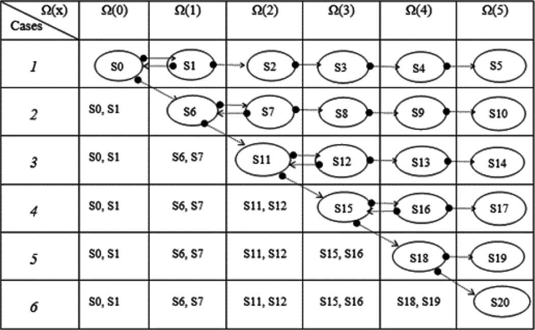
Parameter fixed for each space

For example, in Case 2, the selected Diff value is larger than a state S1 in Ω(1) compare to the state S0 in Ω(0). In this case, after selecting the candidate parameter and its values which is second smallest Diff from S0 and the S1 is re-evaluated with the newly updated sets and the result is saved at S6.

This methodology, each state can be performed once more, so the following additional cost is required. However, we expect to find better results than in e-heuristic greedy, and the performance test for this model will proceed in the next study.

3.5. e-Heuristic Greedy Procedures

The e-heuristic greedy extended from the heuristically-based greedy [11] composed of several functions includes runHadoop(), run-TeraSort(); runTestDFSIO(), runMrBench(). Each function activated by the main, and in these functions, the start () method can be invoked repeatedly supported by the ProcessBuilder Class [15].

for (int i = 0; i < runs, i++) {

  for (int j = 0; j < n, j++) {

    Selected_Par[ ]=DeterminePar

    (IncDec,Default_Par, percentInc,

      parIdx, Low, High);

    if (!(Fixed_par.contains(Selected_Par)){

      runHadoop( );

      runTeraSort( );

      runTestDFSIO();

      runMrBench();

     }

    endfor

  Fixed_Par[idx + 1]= min ext_CPU of OMEGA(i)

  OMEGA(i + 1) = min t_CPU of OMEGA(i)

endfor

ProcessBuilder TestDFSIO_write =

  NewProcessBuilder (“ssh”,

  “hduser@master”, “hadoop”, “jar”,

  “~/hadoop-test-1.1.2.jar”, “TestDFSIO”,

    “write”, “-nrFiles”, fileSize,

   −fileSize”, numFiles);

run_Process (TestDFSIO_write);

run_Process (ProcessBuilder pb) {

  Process process = pb.start ( );

}

ProcessBuilder TestDFSIO_read =

  NewProcessBuilder (“ssh”,

   “hduser@master”, “hadoop”, “jar”,

  “~/hadoop-test-1.1.2.jar”, “TestDFSIO”,

  “read”, “-nrFiles”, fileSize,

  −fileSize”, numFiles);

run_Process(TestDFSIO_read);

run_Process(ProcessBuilder pb) {

  Process process = pb.start( );

}

ProcessBuilder run_TeraGen =

  new ProcessBuilder (“ssh”,

  “hduser@master”, “hadoop”, “jar”,

  “~/hadoop-examples*.jar”,

  “TeraGen”, genSize, “/teraInput”);

run_Process(run_TeraGen);

ProcessBuilder run_TeraSort =

  new ProcessBuilder (“ssh”,

  “hduser@master”, “hadoop”, “jar”,

  “~/hadoop-examples*.jar”,

  “TeraSort”, “/teraInput”, “/teraOutput”);

run_Process(run_TeraSort);

ProcessBuilder run_TeraValidate =

  new ProcessBuilder (“ssh”,

  “hduser@master”, “hadoop”, “job”,

  “-history”, “all”,

  “/teraInput”, “>”,

  “/TeraSort_results.log”

run_Process(run_TeraValidate);

ProcessBuilder run_MrBench =

  new ProcessBuilder (“hadoop”, “jar”,

“~/hadoop-*test*.jar”, “mrbench”,

“-baseDir”,

  processDir, “-numRuns”, numRuns);

run_Process(run_MrBench);

run_Process(ProcessBuilder pb) {

  Process process = pb.start( );

}

4.1. Evaluation Results

The performance of HDFS and MapReduce workloads are measured by TeraSort with Gensize 30 MB, MrBench with five runs, and TestDFSIO with filesize 20 MB. As shown in the following steps, one parameter and its associated values are fixed in each evaluation space. For the display purpose, the Diff value is multiplied by 10 to visualize on the graph.

4.1.2. Parameter evaluation space Ω(0)

In this parameter space Ω(0), the parameter that has the greatest effect on the total execution time is fixed to m.j.s.m.p. with its value 0.709.

• •

  Idx: 4, m.j.s.m.p (mapred.job.shuffle.merge.percent)

• •

  Increased +20%: 0.709, Exec: 45.69, Diff: −12.32 s

• •

  Fixed: {m.j.s.m.p: (0.709)}

• •

  Default: {i.s.m: (100), i.s.r.p: (0.05), i.s.s.p: (0.80), i.s.f: (10), m.j.s.i.b.p: (0.70)}

Figure 4

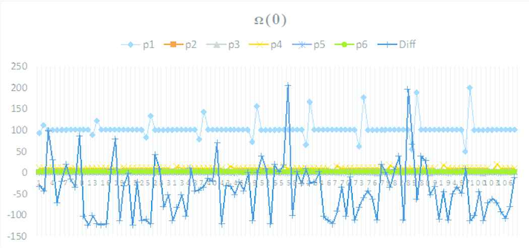
Parameter trends on Ω(0)

4.1.5. Parameter evaluation space Ω(3)

• •

  Idx: 2, i.s.s.p (io.sort.spill.percent)

• •

  Increased +10%: 0.811, Exec: 42.91, Diff: −15.1 s

• •

  Fixed: {m.j.s.m.p: (0.709), i.s.r.p: (0.032), i.s.f: (16), i.s.s.p: (0.811)}

• •

  Default: {i.s.m: (100), m.j.s.i.b.p: (0.70)}

Figure 5

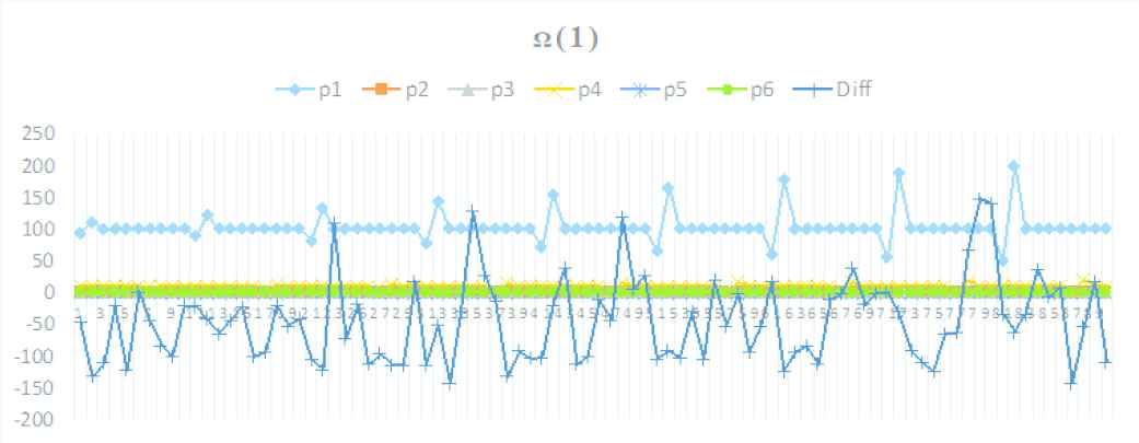
Parameter trends on Ω(1)

Figure 6

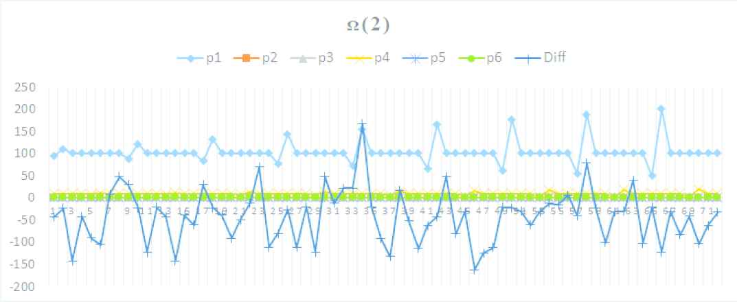
Parameter trends on Ω(2)

4.2. Total Benchmarking Space Trend Analysis

Through the e-heuristic greedy algorithm, parameters are identified for each evaluation space as shown in Table 6. We did not find the most optimal parameter set in Ω(5) at the last stage, but fortunately we could identify the set that optimizes performance among the six spaces in Ω(4) with a parameter set and values {m.j.s.m.p: (0.709), i.s.r.p: (0.032), i.s.f: (16), i.s.s.p: (0.811), i.s.m: (66), m.j.s.i.b.p: (0.70)} to minimize execution time of −17.2 s. It can be said that the local minimum value selected at each stage contributed to finding a globally optimal value.

Figure 7

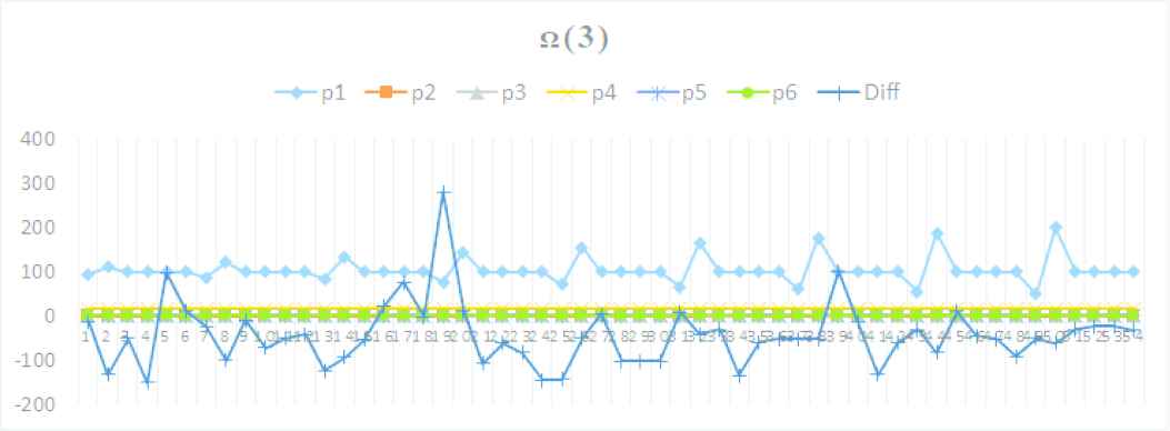
Parameter trends on Ω(3)

Figure 8

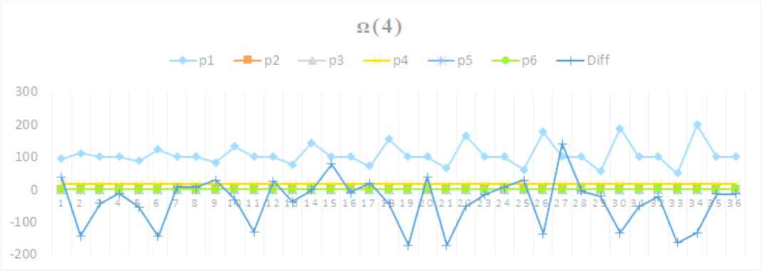
Parameter trends on Ω(4)

Figure 9

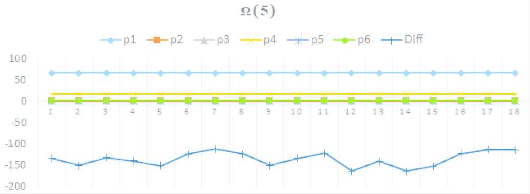
Parameter trends on Ω(5)