
MLP and CNN-based Classification of Points of Interest in Side-channel Attacks
- DOI
- 10.2991/ijndc.k.200326.001How to use a DOI?
- Keywords
- Point of interest; forward difference; trace; multi-layer perceptron; convolutional neural network
- Abstract
A trace contains sample points, some of which contain useful information that can be used to obtain a key in side-channel attacks. We used public datasets from the ANSSI SCA Database (ASCAD) as well as SM4 traces to learn whether a trace consisting of Points of Interest (POIs) have a positive effect using neural networks. Different methods were used on these datasets to choose POI or transform the traces into Principal Component Analysis (PCA) traces and forward-difference traces. The results show that two datasets are combined in different ways that improve the classification using neural networks. For example, for the ANSSI SCA database, PCA is a better approach to compress a 700-dimensional trace into a 100-dimensional trace. For SM4 traces, the amount of traces required can be reduced in side-channel attacks subsequent to forward-difference transformation.
- Copyright
- © 2020 The Authors. Published by Atlantis Press SARL.
- Open Access
- This is an open access article distributed under the CC BY-NC 4.0 license (http://creativecommons.org/licenses/by-nc/4.0/).
1. INTRODUCTION
Side-channel attack was proposed by Kocher et al. [1]. It is a form of physical attack that can be used to obtain an encryption key from unintended leakage information, or energy consumption [2], and collected using hardware such as resistance and oscilloscopes. The leakage information can be analyzed using Differential Power Analysis (DPA) [1], Correlation Power Analysis (CPA) [2], zero value attacks [3], profiling attacks [4], mutual information analysis [5], template analysis [6] etc., to obtain the key used to encrypt plain texts. Neural networks have gained considerable popularity in recent times owing to their application in different fields. They are now being used [7,8] in analyzing leakage information. As they can be used to learn characteristics from traces in training datasets, whereby the trained model is used to classify traces in test datasets to obtain the key.
A trace is defined as follows: “a set of power consumption or electromagnetic power radiation during a cryptographic operation.” [1]. Figure 1 shows a trace comprising 2 million sample points from a STM32F103RCT6 that performs an SM4 encryption, with 32 rounds clearly visible. The starting point for the encryption is close to 0.3 in the sample points, whereas its end point approaches 0.8.
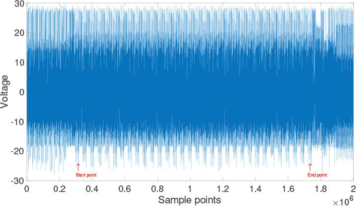
A trace showing 32-round encryption in SM4.
Figure 2 shows traces whose Hamming Weights (HWs) are different from those in the training datasets, which causes variations in voltage consumption at different sample points. Each trace has such unique characteristics that an attacker can determine the key that was used for encryption (Figure 3).
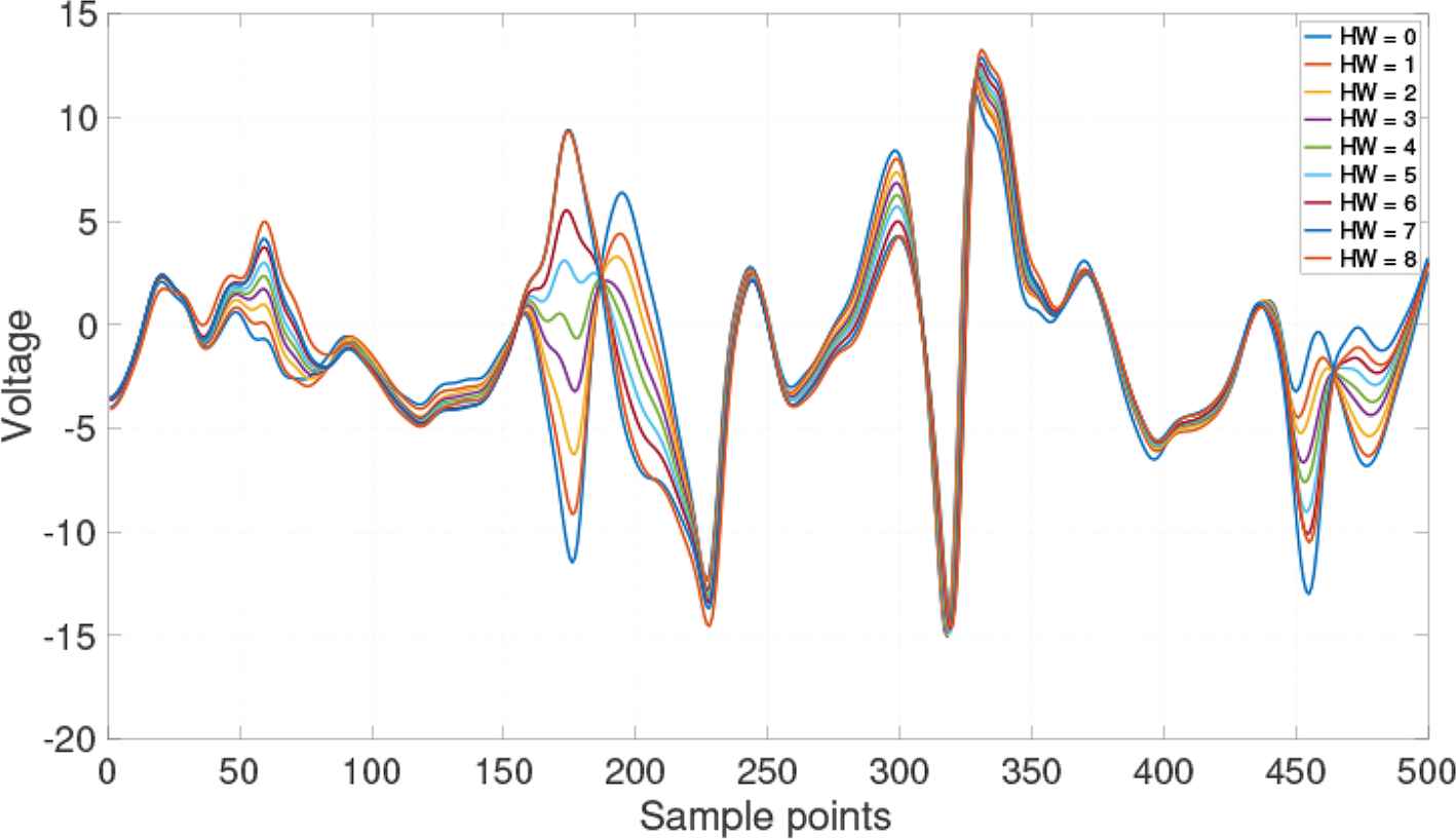
Different hamming weights in SM4 traces.
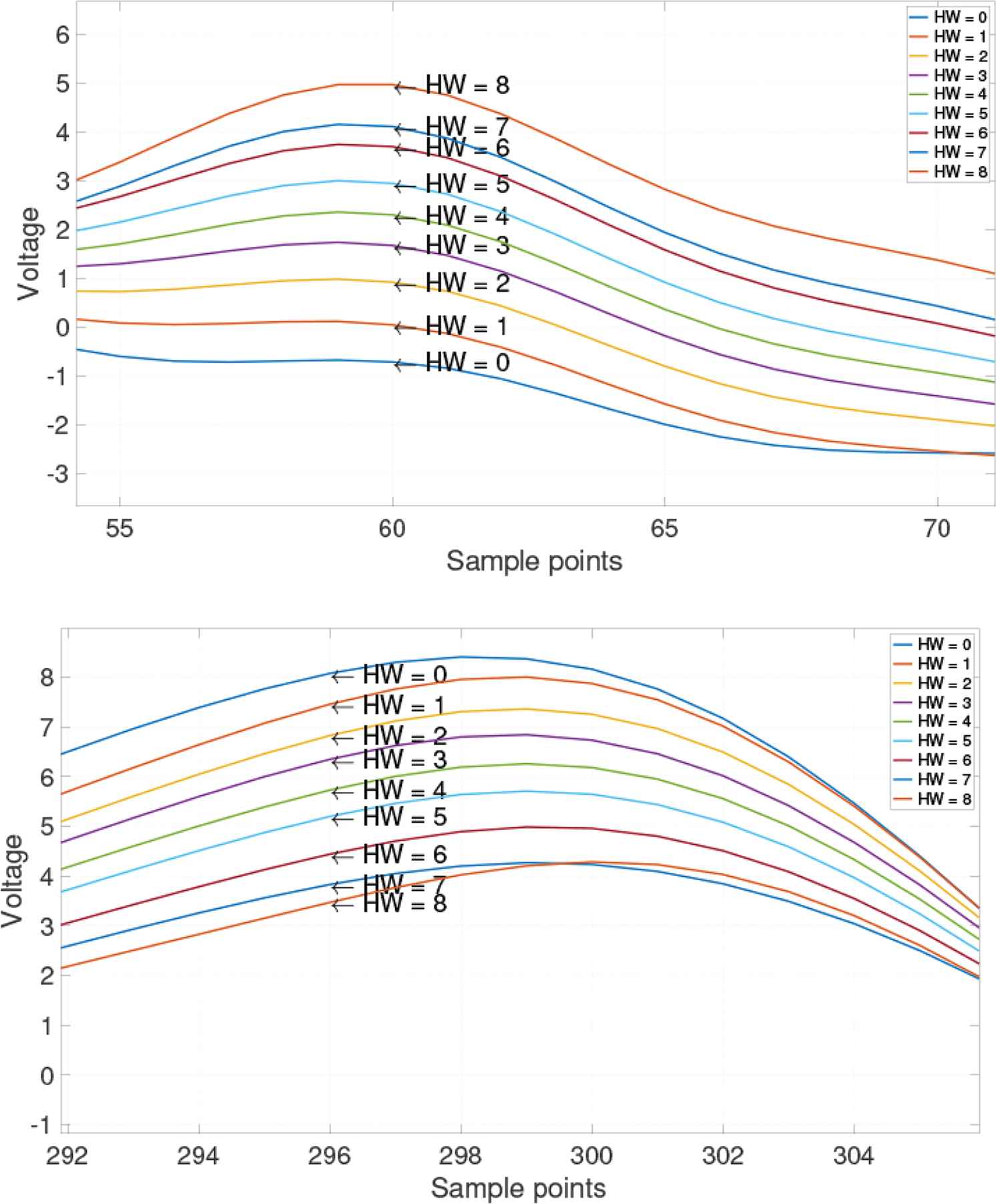
Hamming weights in the traces.
When viewed at a higher resolution, it is obvious from Figure 2 that the trace for voltage consumption at the trace for HW = 8 is greater than that at HW = 0 at the 60th sample point; however, this may not hold true for all observations. In contrast, at the 296th sample point, an entirely opposite trend is observed for the consumptions.
In addition to the energy consumption, new types of leakages were found, including the duration of encryption [9], electromagnetic radiation [10], sound leakage [11], photon radiation [12]. Computer security experts, Genkin et al. [13] discovered new sidechannel leakages in 2015. They demonstrated the extraction of secret decryption keys from laptops and computers, by nonintrusively measuring the electromagnetic emanations for a few seconds from a distance of 50 cm. The attack can be executed using inexpensive and readily-available equipment: a consumer-grade radio receiver or a software-defined radio USB dongle. Three years later, they discovered another leakage [14]: the visual content displayed on a user’s screen leaks onto the faint sound emitted by the screen. This sound can be gathered by ordinary microphones built into webcams or screens, and is inadvertently transmitted to other parties, e.g., during a videoconference call or archived recordings.
2. SM4 BLOCK CIPHER ALGORITHM
The National Encryption Algorithms are domestic commercial cryptographic algorithms recognized by the State Cryptography Administration of China. It contains a series of algorithms, including symmetric encryption (SM1, SM4, SM7, ZUC), ellipticcurve cryptography (SM2, SM9), and hash algorithm (SM3).
SM4 (formerly SMS4) is a block cipher, that was released on March 21, 2012 (there is an English edition of SM41 translated by W. Diffie and G. Ledin). SM4 has an input length of 128 bits and a key length of 128 bits. Both the encryption and the key expansion algorithm use the 32-round nonlinear iterative structure, and the round key is generated through expansion of the initial key. Decryption and encryption have the same structure; however the order in which the round key is used is reversed, hence, the decryption round key is in reverse order to the encryption round key.
First-round encryption is presented from Figure 4:
- (i)
A 128-bit plaintext is equally divided into 32-bit X0, X1, X2, and X3 from left to right.
- (ii)
X1 ⊕ X2 ⊕ X3 ⊕ the first-round key (Rk).
- (iii)
Divide the Exclusive OR (XOR) result from left to right into four 8-bit intermediate values: V0, V1, V2 and V3.
- (iv)
V0, V1, V2 and V3 are substituted by the exact same S-box.
- (v)
Combine the four 8-bit results for the S-box into a 32-bit V4.
- (vi)
V4 performs a nonlinear transformation L.
- (vii)
The output of L ⊕ X0 to get X4.
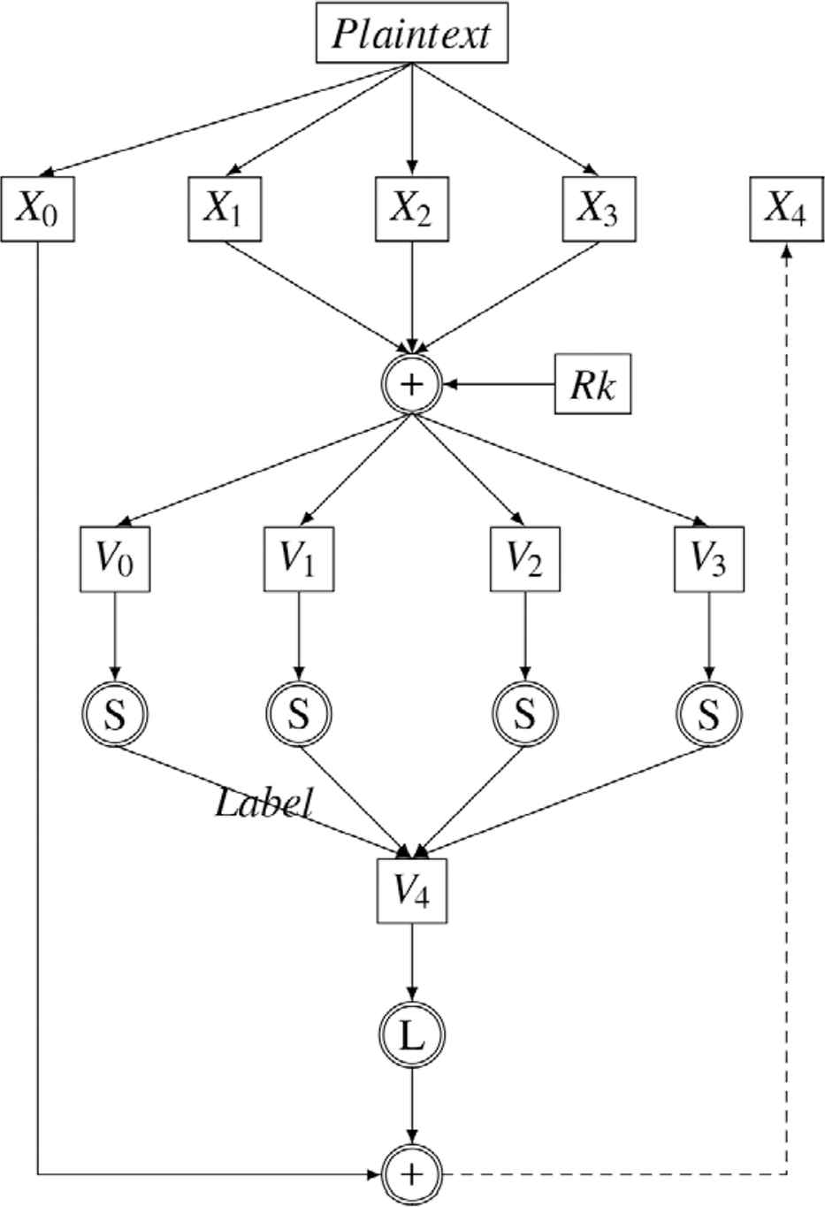
The first round encryption of SM4.
In the second-round encryption, X2 ⊕ X3 ⊕ X4 ⊕ the second-round key (Rk). After following step (iii) to step (vii), X5 will be generated.
3. COLLECTING SM4 TRACES
Collecting traces is an important step in side-channel attacks. The process involves recording physical information such as power consumption and electromagnetic radiation using hardware equipment while the cryptographic algorithm is running. The software and hardware parameters used and the collection process directly affects the signal-to-noise ratio of the traces, which in turn affects the final results.
The power supply must ensure that the supply voltage is stable during the leakage collection process. The power must be able to drive the cryptographic device to function effectively, and the noise needs to be as low as possible. An oscilloscope can be used to check if the voltage waveform of the power supply contains noise or glitches. If the device itself has no supporting power supply or has poor quality of supporting power supply, an external power device should be connected to the encryption device.
3.1. Preparation
The traces used in this study were collected from the STM32F103RCT6 in Figure 5, a single-chip microcomputer, running the SM4 code. During the encryption process, the electromagnetic probe collects electromagnetic signals outside the chip.

STM32F103RCT6 is on testing.
The key is 0x 00 11 22 33 44 55 66 77 88 99 AA BB CC DD EE FF, meanwhile, a trigger was added to the program, and code samples to convert the value stored in the register to zero was added to the SM4 code. This increases the Hamming distance in the leaked information. Besides the single-chip microcomputer, an oscilloscope was used to observe the traces. The sampling frequency was 10 Ghz/s.
The trigger signal (the yellow wave in Figure 6) was generated by changes in voltage (the green one) on a pin of the STM32F103RCT6 to assist the oscilloscope to locate the starting point for the encryption. Meanwhile, the trigger signal can be set high when no encryption process is involved, then set low before the cryptographic algorithm is run, and low again after the encryption is completed.
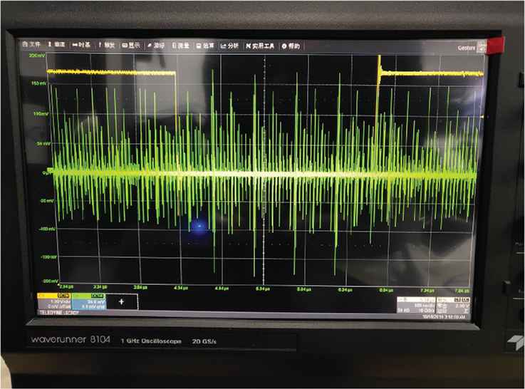
Oscilloscope is running.
3.2. Collection Routine
- (i)
After the single-chip microcomputer STM32F103RCT6 and the oscilloscope are correctly connected, the computer sends a random plaintext to the MicroController Unit (MCU) (single-chip microcomputer). A total of 30,000 random plaintexts were sent at the end of the collection.
- (ii)
The MCU encrypts the plaintext with SM4 algorithm and sends the ciphertext back to the computer. The electromagnetic probe is placed on the chip to collect electromagnetic wave. At the same time, the trigger signal is also transmitted to the oscilloscope.
- (iii)
With the help of the trigger used to adjust the oscilloscope, it receives all the waveforms during the encryption process. The first-round waveform is found and enlarged on the horizontal axis. If the traces are just for experimentation, the sample points after the first round do not need to be recorded.
- (iv)
The traces collected by the oscilloscope are sent to the computer for a series of preprocessing, including low-pass filtering and removing high frequency noise. Subsequently, a fragment of the traces from the 300th to 350th sample points are selected as a reference to align all the traces. Some of the traces that were not properly aligned were deleted, finally leaving 29,494 traces.
- (v)
To accurately locate the first round of encryption, the collected traces were first analyzed using CPA; the target is the first S-box transformation. The CPA results show that at about the 173th sample point in all traces, the first eight bits of the Rk round key was known to be 0xd7.
- (vi)
Select an interval around the 173th sample point to include the traces in the S-box transformation. Save the traces in this range as the training datasets to be used in the neural network. The traces used in this paper contains 500 samples around the 173th sample point.
- (vii)
The label of each trace is the output of the S-box. According to the 10:1 principle, 20,000 traces were randomly selected as training datasets, while the remaining 2000 traces were used as testing datasets (Figure 7).
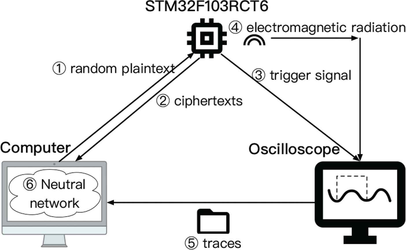
Data transmission.
For packet encryption, traces for the S-box transform or similar nonlinear transforms are often collected. The data in this paper is for the first S-box transform whose input is V0 in the first round of SM4 encryption. The label of a trace is the output from the S-box (Label in Figure 4).
4. TRANSFORMATION OF THE TRACES
When using neural networks to classify traces collected in side-channel attacks, the focus is usually on the performance of the neural networks employed and their optimization, and the transformation of the traces is usually ignored. The assertion that “dimensionality reduction never raises the informativeness of the data” [15,16] may not be entirely accurate in my opinion. In this section, different Points of Interest (POIs) are extracted from the ANSSI SCA database (ASCAD)2 traces to form a new type of traces. The order of the POI is the same as the order in ASCAD. These POI shorten the lengths of traces or reduce their dimensions. To compare with POI traces, ASCAD traces are transformed through Principal Components Analysis (PCA) [17]. PCA traces have the same lengths as those of POI traces.
4.1. POI-traces in ASCAD and SM4
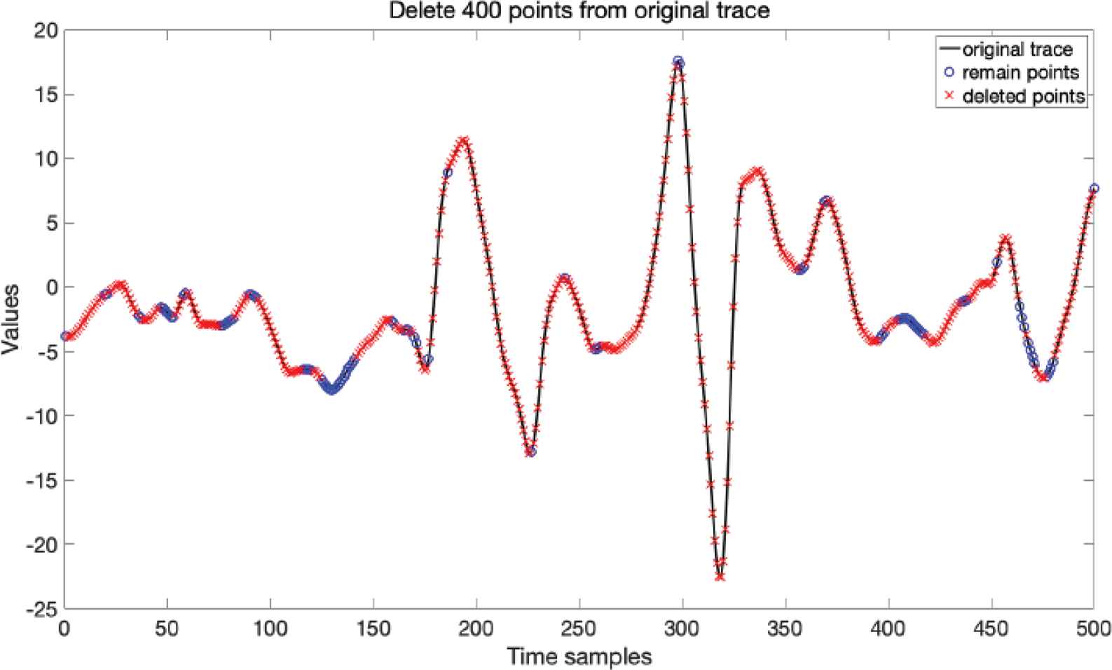
A single trace from ASCAD is composed of 700 sample points. 200 sample points were removed from an ASCAD - trace700, leaving 500 POI to form a POI – trace500 in Figure 8. Figure 9 shows an ASCAD - trace700 after 400 sample points were removed to leave 300 POI. The points were deleted from lines in which the absolute value of the slope is large, because Figure 2 and the CPA results for SM4 traces show that such inflection points are important for obtaining the key from traces and that traces with different HWs have their unique characteristics at the inflection points in Figure 3. With these characteristics, the key can be derived from a trace. The SM4 traces in Figure 2 were transformed by the same method, and there are POI - trace100 in Figure 10, POI - trace700, POI - trace300, POI - trace400.
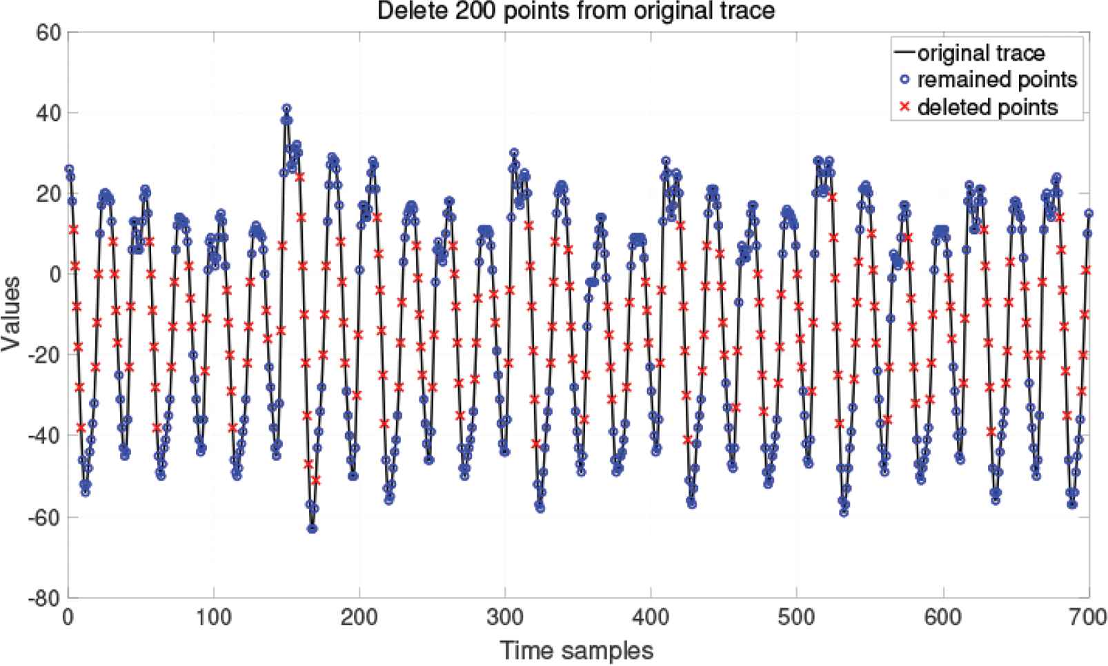
A POI-trace contains 500 sample points.
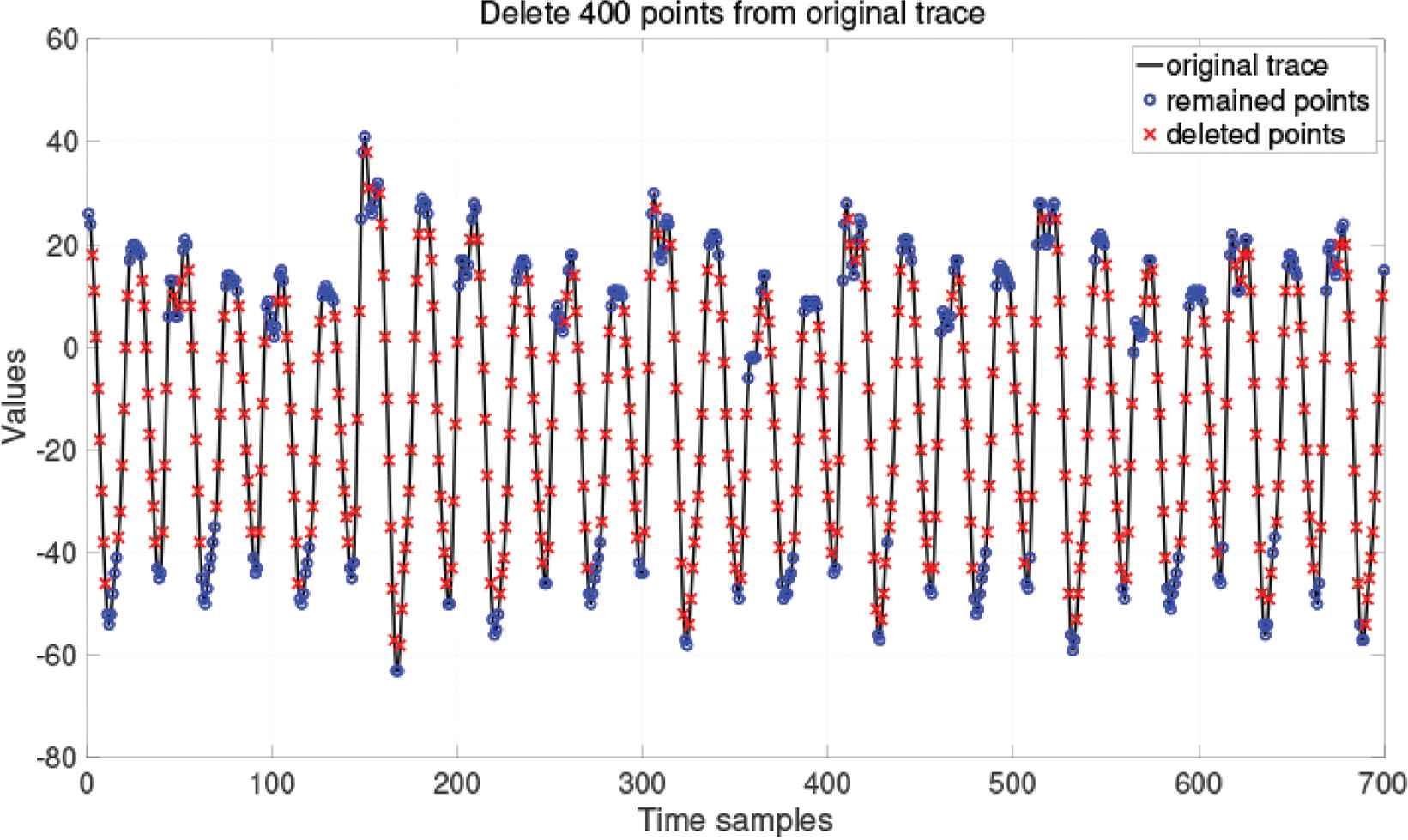
A POI-trace contains 300 sample points.
A SM4 POI-trace containing 100 sample points.
If we let Δx and Δy be the distances (along the x and y axes, respectively) between two points on a curve, then the slope is given by,
Since traces are discrete data, Δx must be an integer. Δx = 1 in (1) to select the POI.
To some extent, a trace can be considered as a continuous curve formed by several discrete points. To preserve the sample points at the “peak” and “valley” positions or inflection points in the trace, the remaining sample points were deleted. If the traces from ASCAD could be regarded as a continuous and differentiable curve f(x), and x is a sample point, x ∈ [1, 700], the POI would be selected to preserve sample points whose f′(x) = 0, or |f′(x)| ≈ 0.
4.2. Principal Components Analysis in ASCAD
The curves in Figure 11 were superimposed by 1000 traces in ASCAD. The PCA traces in Figure 12 were transformed with the same 1000 traces using PCA [18]. The amplitude or value of the PCA traces decreases after 20 sample points, while the amplitude of the first 20 points drops rapidly. The traces in ASCAD are expressed as ASCAD – traces = (t1, t2, t3…t700), where ti is the value of the ith sample point. The PCA - traces = (p1, p2, p3…p700), where the length of the transformed traces is still 700, PCA - trace100 = (p1, p2, p3…p700) and PCA - trace100 selects the first 100 points from the PCA-trace, PCA - trace200 = (p1, p2, p3…p200), etc.
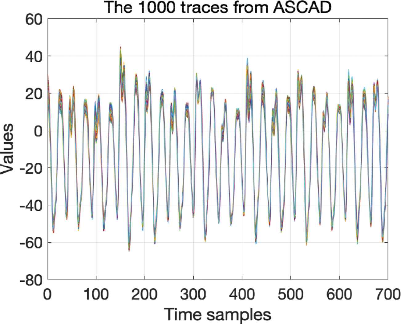
1000 original traces from ASCAD.
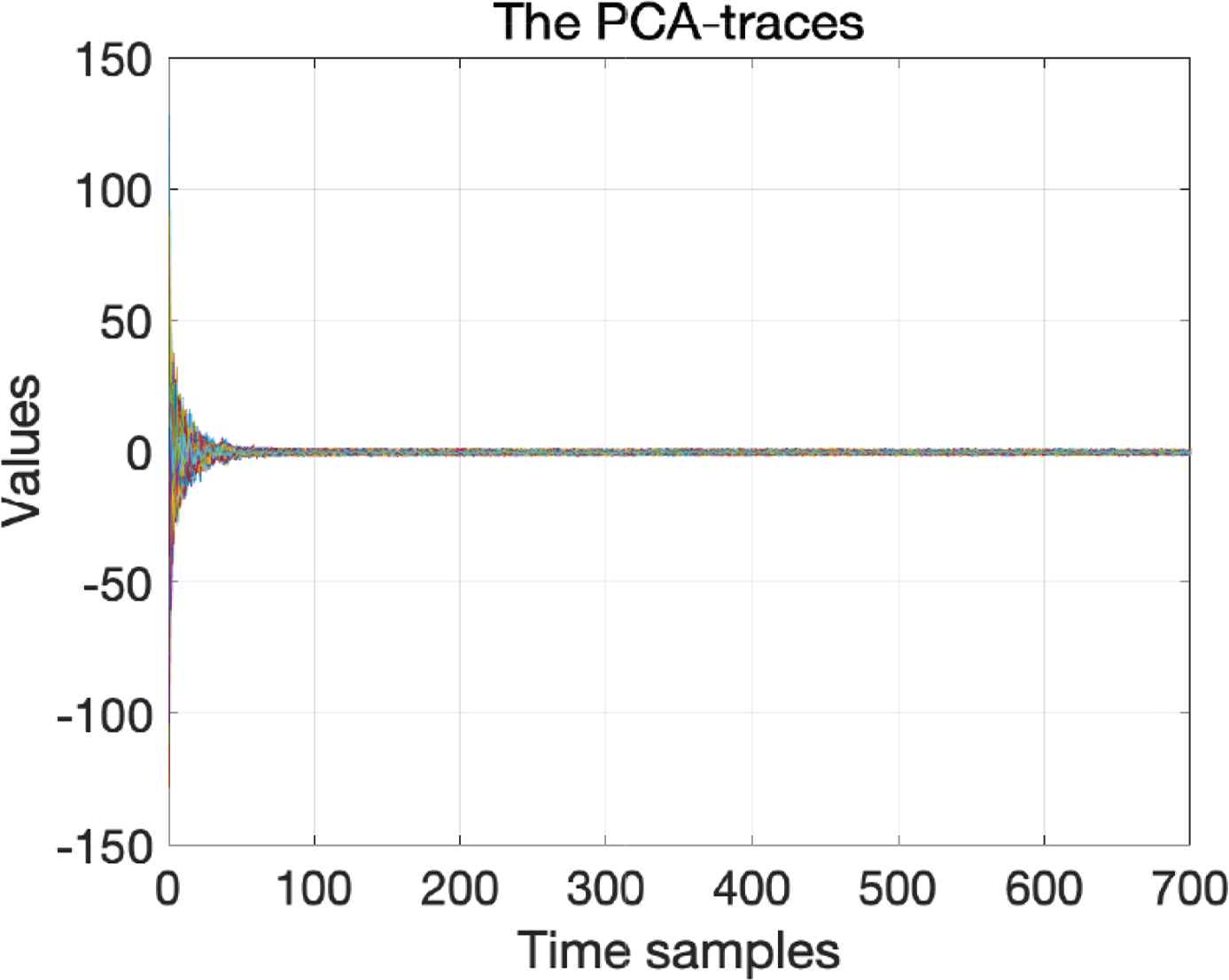
The 1000 PCA-traces.
4.3. Forward Difference Traces in SM4
Now that the deleted points in ASCAD are in the steep lines, the slope in a trace may affect the result in SCA. A forward difference is an expression of the form:
Since the traces are discrete, the h in “Equation (2)” must be an integer. In forward difference SM4 traces, we tried h = 1, h = 2,…, h = 6, h = 7. For example, there are two SM4 traces: T1(x) = [1,2,4,3,2], T2(x) = [1,0,−2,−1,1], the forward difference traces represent Tfd1(x) = [1,2,−1,−1], Tfd2(x) = [−1,−2,1,2], where h = 1.
5. RESULTS
The ASCAD training datasets for POI traces and PCA traces with both containing 50,000 traces were fed into two neural networks: Multi-Layer Perceptron (MLP) [19] and Convolutional Neural Networks (CNN) [20]. We compared the performance of the MLP and CNN models using classification results from testing datasets containing 10,000 traces. Similarly, we compared results obtained from the MLP and CNN classification for the original aligned traces from ASCAD with the best results for PCA traces and POI traces. A root mean square propagation optimizer was used in the MLP and CNN. It keeps a moving average of the squared gradient for each weight [21],
The evaluation method followed the scheme in Benadjila et al. [2], where ‘rank’ is: when using t traces for classification (t is the minimum sum of traces required to obtain the real key) traces, 256 potential subkeys with a length of 1 byte respectively yield a probability vector,
where ε is a small positive number such as 0.00001. After sorting all the probabilities in descending order in
If t < n,
When t ≥ n,
This can be considered that rank(t) will not increase after n traces and that the key from the datasets will remain unchanged. This special point, t = n is denoted as η. In ASCAD, η ∈ [1, 10000], but in SM4 traces, η ∈ [1, 2000]. When η is greater than the maximum number, there is no correct result since the correct key cannot be obtained in the testing dataset.
5.1. Classification Results for ASCAD using CNN
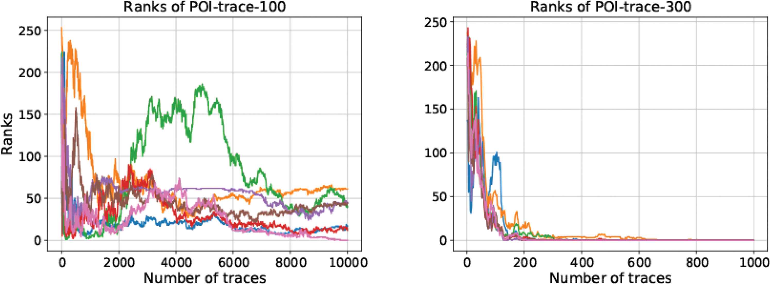
Select 100, 200, 300, 400, 500, and 600 points of interest from ASCAD to form different POI traces. Since the article has a limited length, only two results are given here. Two kinds of POI traces containing 100 and 500 POI were classified using CNN, as shown in Figure 13. There are seven curves in each graph, each corresponding to the result of identical parameters in the models. Figure 13 shows that the results for POI - trace100 were worse than those for the POI - trace500 in the classification using CNN.

Ranks of POI - trace100 and POI - trace500.
The classification results improve as the number of points of interest increases. However, this is not always the case. An anomaly was observed in the results for POI - trace500 which were slightly better than those for POI - trace600.
The lengths of the PCA traces were the same as those of the POI-trace, with 100, 200, …, 600 sample points and seven curves in every graph, as shown in Figure 14. But a curve rise up in the results of both PCA - trace100 and PCA - trace400. When the curves are observed at higher resolutions, a slight difference is noticed between the two similar curves, though they look alike initially. The classification results for the PCA - trace600 are slightly worse than those for both the PCA - trace100 and PCA - trace400; however, the curves do not always ascending. The PCA traces do not offer better results while there are more sample points in single trace. The average results for the POI and PCA traces classified using CNN are shown in Table 1.
Ranks with PCA - trace100 and PCA - trace400.
| Length | POI mean η | PCA mean η |
|---|---|---|
| 100 | 7497 (*) | 2440 (*) |
| 200 | 7390 (*) | 2563 |
| 300 | 186 | 1673 |
| 400 | 208 | 2805 (*) |
| 500 | 139 | 1305 (*) |
| 600 | 264 | 1781 |
Mean η for different traces classified using CNN
The values at the mean η for POI and PCA in Table 1 were calculated by averaging the η for the seven results in each graph. When a ‘(*)’ behind a number, at least one rank cannot equal to 0 finally. Since there are only 10,000 traces in ASCAD testing dataset, η = 10000 when there is a ‘(*)’.
The characteristics of the PCA traces were different from those of the POI traces. As shown in Figures 8 and 9, the values of PCA traces remain unchanged after extracting the POI, though some points were deleted from the original traces. The PCA traces in Figure 12 become a different kind of trace completely and the values also change. After 20 sample points, the difference of the PCA traces becomes very small, which may be detrimental to learning the characteristics of the PCA traces using neural networks.
To compare the results of PCA traces and POI traces using CNN, when a trace has only 100 sample points, using PCA traces is obviously better than other kinds of traces. The classification results obtained using the POI traces improves as the number of sample points increases, but the results obtained with the PCA traces are not improved. The computational capability is not enough to use neural networks for classification, hence, only traces with small dimensions can be fed into it. PCA can significantly reduce the dimensions of a trace to ensure that the classification results are acceptable. Otherwise, when it is possible to train with high-dimensional traces, it is better to use POI traces when there is only a small number of traces in the training dataset, however, high-dimensional POI traces are required for obtaining the correct key.
5.2. Classification Results for ASCAD using MLP
Classification results for 100 and 300 POI traces fed into the MLP (Figure 15). When there are only 100 POI, the correct key cannot be obtained using MLP. The value of a rank is bigger, and keep away from the X-axis while the trace containing 200 POI, which means the classification results are even worse. The classification results obtained for POI - trace300 are significantly better than those obtained for POI - trace100 and POI - trace200. However, the POI - trace600 yield poor results when MLP is used; it is either the performance of the neural network is poor, or there are some “redundant” points in the 600 points, which yields the poor classification results (Figure 16).
Ranks with POI - trace100 and POI - trace300.

Ranks with PCA - trace100 and PCA - trace400.
The classification results for the PCA traces using MLP is different from the results for PCA traces using CNN. A small number of PCA traces can be used to obtain the correct key using MLP when a single trace has a few sample points. This may not be possible if the PCA traces were classified using CNN. Hence, MLP is a better model than CNN for classifying the PCA traces Table 2.
| Length | POI mean η | PCA mean η |
|---|---|---|
| 100 | 9965 (*) | 238 |
| 200 | 10,000 (*) | 498 |
| 300 | 1533 | 1601 |
| 400 | 4503 | 819 |
| 500 | 2933 | 346 |
| 600 | 1760 | 973 |
Mean η of different traces using MLP
5.3. The Best Result in ASCAD using CNN or MLP
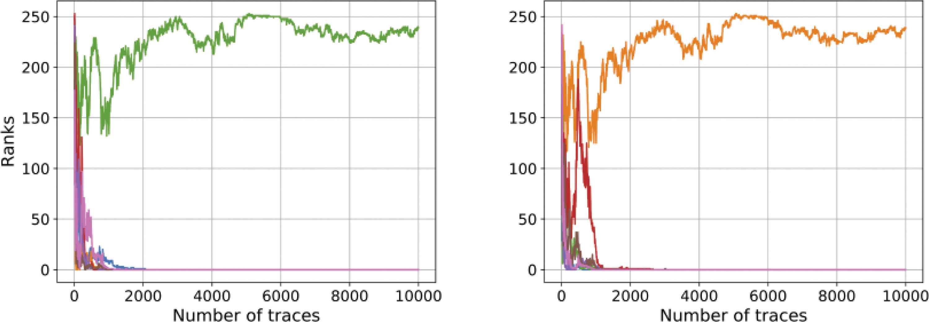
The left portion of the graph in Figure 17 shows the best classification results obtained using MLP with three kinds of traces whereas the right graph represents the best results using CNN. ‘Best’ here implies that among all the results, it requires the minimum number of traces to obtain the correct key. Table 3 shows the number of sample points in a trace and the minimum η in the best results. Figure 17 and Table 3 show that for the three trace lengths and two neural networks, the best classification result is obtained with the PCA - traces100 classified using MLP. The classification results for POI - traces300 using CNN are similar to the best one. In reality, the computational requirements are different; PCA - traces100 using MLP requires less computational resources than POI - traces300 using CNN. However, both the PCA traces and the POI traces offer better results than the original traces obtained in ASCAD for performing side-channel attacks using neutral networks.
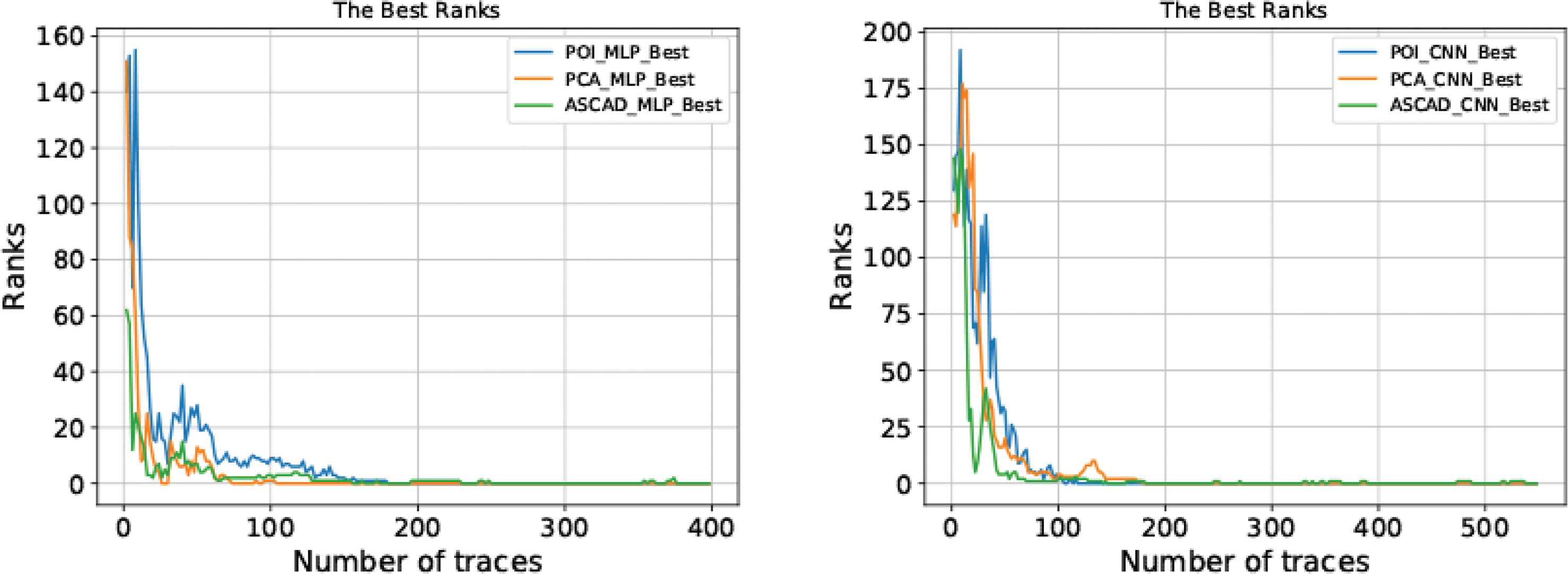
The best ranks.
| Dataset-length | MLP η-min |
| ASCAD-700 | 538 |
| POI-300 | 118 |
| PCA-500 | 180 |
| Dataset-length | CNN η-min |
| ASCAD-700 | 376 |
| POI-500 | 180 |
| PCA-100 | 104 |
Minimum values of η
5.4. SM4
5.4.1. Ranks of SM4 Traces
The traces in SM4 dataset is shown in Figure 2. Some statements in the SM4 code worsens the leakage, which is due to the large HWs at some sample points. The classification results for SM4 are much better than those for ASCAD. Figure 18 shows the classification results for SM4 using MLP and CNN. It can be seen that about 30 traces are required for the two models to make rank equal to 0. Moreover, when rank is not equal to 0, its value tends to fluctuate with increasing number of traces.
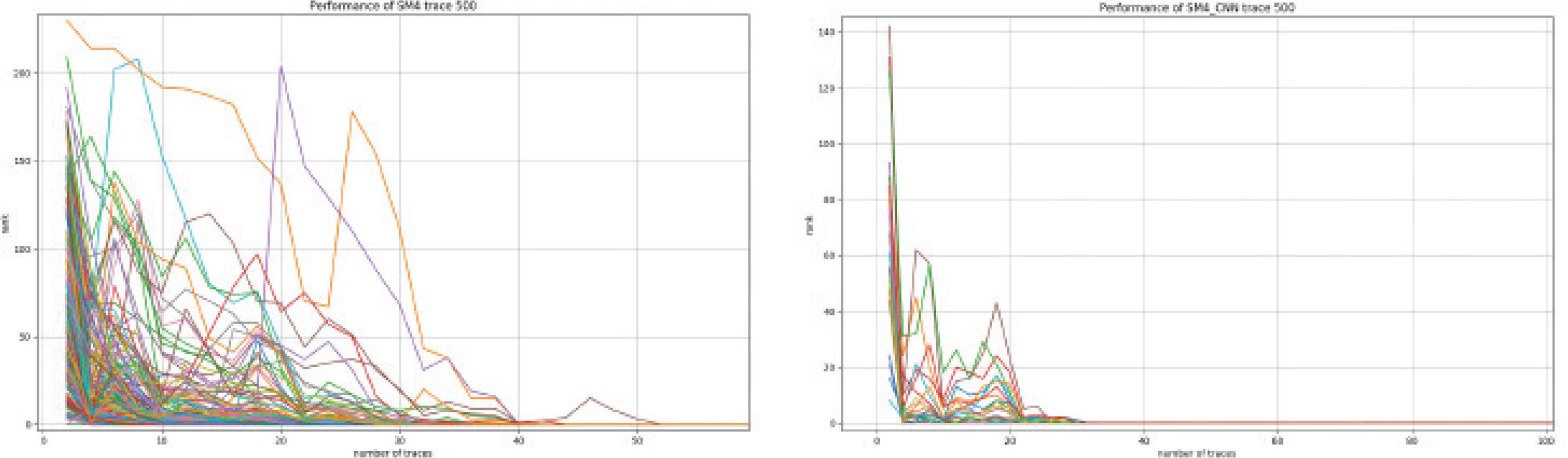
Ranks of SM4 traces by using MLP and CNN.
5.4.2. Ranks for SM4 POI-100 Traces
The SM4 traces are for selected PI. The original traces contain 500 sample points, where the number of POI are 100, 200, 300, 400. The classification results are shown in Figure 19 for 100 POIs.
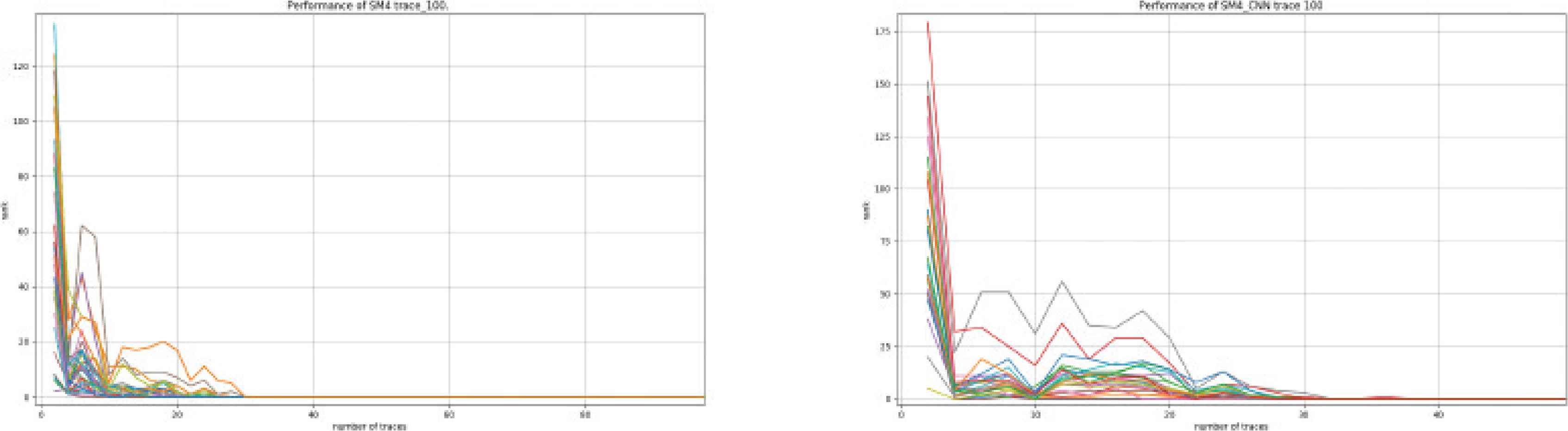
Ranks of POI-100 traces by using MLP and CNN.
5.4.3. SM4 Ranks for Forward-difference Traces
MLP and CNN were also used to classify the SM4 forward differential traces. The MLP classification results are shown in the upper figure of Figure 20. The top row of each picture represents the results for 0–3 order forward differences while the bottom row represents the results for 4–7 order forward difference. The classification results significantly improve and the fluctuation of rank vanishes when forward difference is applied to the traces, which is quite different from the original traces and the POI traces for SM4. The original traces for SM4 requires about 30 or 40 traces to make rank equals 0, but MLP requires only 10 traces to achieve the same result for first-order differential traces. Second-, third-, and fourth-order differential traces all have similar results. However, starting from the fifth-order forward difference, the results begin to deteriorate. By the seventh-order, the rank could not be equal to 0 even if 2000 traces are used in the testing datasets. The results obtained using CNN are similar to those obtained using MLP, as shown in the lower part of Figure 20. However, the classification results for the first-order forward difference for MLP was significantly improved, while the result obtained using CNN begins to improve in the second-order. Meanwhile, the sixth-order forward difference classification results for CNN could not be made equal to 0.
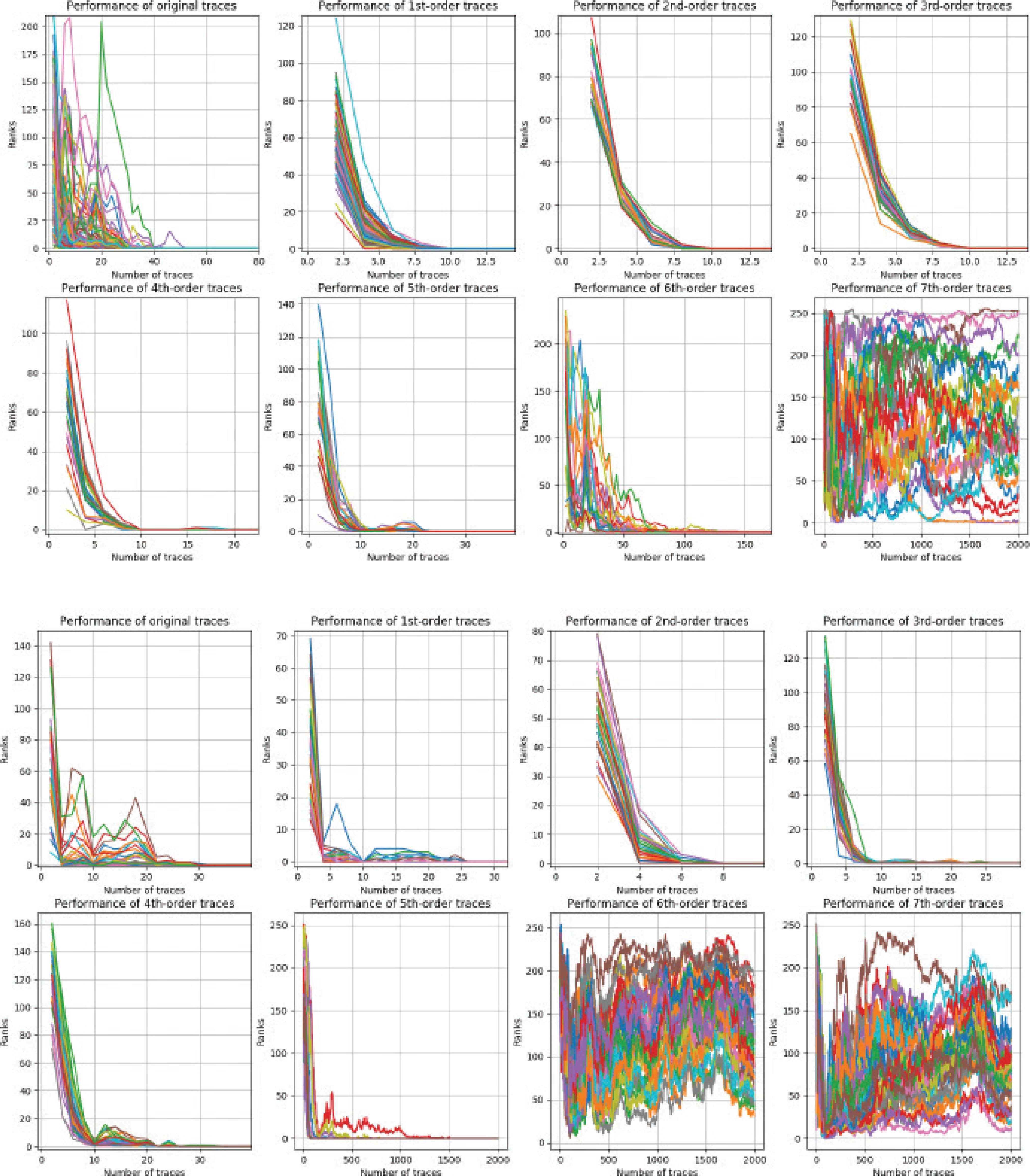
Ranks of forward difference traces using MLP and CNN.
6. CONCLUSION
We used three methods to transform original traces to new ones that are fed into neural networks. Results obtained in ASCAD show that PCA transformation is better than the original traces. A trace containing 700 samples was used to obtain the key points in ASCAD. This can also be achieved using PCA - traces100 with MLP; however, the number of neurons in the neural network is smaller and the training time is shorter. Out results show that MLP is more suitable for PCA traces than CNN. However, POI traces achieves better results if CNN used. The results obtained after transforming SM4 traces through one to seven order forward difference were better than the original traces obtained using MLP or CNN. We aimed to study the influence of pretreatment on traces, so the number of layers or neurons, or the type of activation function was not the focus of this work, hence, they were not considered in this paper. There were uncontrollable factors in the training process that can affect the performance of the neural networks. For instance, since the initial values of the weights were randomly generated, they have a strong influence on the results. The main goal of this work was to show that it is better to feed shorter traces to neural networks for side-channel attacks, which also improves the classification results.
CONFLICTS OF INTEREST
The authors declare they have no conflicts of interest.
ACKNOWLEDGMENTS
This work is supported by
Footnotes
SMS4 Encryption Algorithm for Wireless Networks. https://eprint.iacr.org/2008/329.pdf.
ANSSI. ASCAD database. https://github.com/ANSSI-FR/ASCAD, 2018.
REFERENCES
Cite this article
TY  - JOUR
AU  - Hanwen Feng
AU  - Weiguo Lin
AU  - Wenqian Shang
AU  - Jianxiang Cao
AU  - Wei Huang
PY  - 2020
DA  - 2020/04/17
TI  - MLP and CNN-based Classification of Points of Interest in Side-channel Attacks
JO  - International Journal of Networked and Distributed Computing
SP  - 108
EP  - 117
VL  - 8
IS  - 2
SN  - 2211-7946
UR  - https://doi.org/10.2991/ijndc.k.200326.001
DO  - 10.2991/ijndc.k.200326.001
ID  - Feng2020
ER  -