
Compositional Stochastic Model Checking Probabilistic Automata via Assume-guarantee Reasoning
- DOI
- 10.2991/ijndc.k.190918.001How to use a DOI?
- Keywords
- Stochastic model checking; assume-guarantee reasoning; symmetric assume-guarantee rule; learning algorithm; probabilistic automata
- Abstract
Stochastic model checking is the extension and generalization of the classical model checking. Compared with classical model checking, stochastic model checking faces more severe state explosion problem, because it combines classical model checking algorithms and numerical methods for calculating probabilities. For dealing with this, we first apply symmetric assume-guarantee rule symmetric (SYM) for two-component systems and symmetric assume-guarantee rule for n-component systems into stochastic model checking in this paper, and propose a compositional stochastic model checking framework of probabilistic automata based on the NL* algorithm. It optimizes the existed compositional stochastic model checking process to draw a conclusion quickly, in cases the system model does not satisfy the quantitative properties. We implement the framework based on the PRISM tool, and several large cases are used to demonstrate the performance of it.
- Copyright
- © 2019 The Authors. Published by Atlantis Press SARL.
- Open Access
- This is an open access article distributed under the CC BY-NC 4.0 license (http://creativecommons.org/licenses/by-nc/4.0/).
1. INTRODUCTION
Formal verification can reveal the unexposed defects in a safety-critical system. As a prominent formal verification technique, model checking is an automatic and complete verification technique of finite state systems against correctness properties, which was pioneered respectively by Clarke and Emerson [1] and by Queille and Sifakis [2] in the early 1980’s. Whereas model checking techniques focus on the absolute correctness of systems, in practice such rigid notions are hard, or even impossible, to ensure. Instead, many systems exhibit stochastic aspects [3] which are essential for among others: modeling unreliable and unpredictable system behavior (message garbling or loss), model-based performance evaluation (i.e., estimating system performance and dependability) and randomized algorithms (leader election or consensus algorithms). Automatic formal verification of stochastic systems by model checking is called stochastic model checking or probabilistic model checking [4].
Stochastic model checking algorithms rely on a combination of model checking techniques for classical model checking and numerical methods for calculating probabilities. So, stochastic model checking faces more severe state explosion problem, compared with classical model checking [5]. There are some works to deal with this problem through bounded probabilistic model checking [6], abstraction refinement [7], compositional verification [8] and so on. The crucial notion of compositional verification is “divide and conquer”. It can decompose the whole system into separate components and conquer each component separately. The compositional verification techniques include assume-guarantee reasoning [9], contract-based methods [10] and invariant-based methods [11]. This paper focuses on assume-guarantee reasoning, which is an automatic method of compositional verification. To account for the relationship between the whole system and its different components, assume-guarantee reasoning gives some rules, which can change the global verification of a system into local verification of individual components.
Theoretically speaking, applying the assume-guarantee reasoning into stochastic model checking is a feasible way to solve the state explosion problem. There is some research work done in this direction [12–15]. We argue that applying the assume-guarantee reasoning into stochastic model checking should solve the following four issues, which is named as AG-SMC problem: (1) How to generate appropriate assumptions. (2) How to check the assume-guarantee triple. (3) How to construct a counterexample. (4) How to verify a stochastic system composed of n (n ≥ 2) components.
1.1. Related Work
According to the generation type of assumptions, we divided the existed work into two categories.
1.1.1. Manual interactive assumption generation
On the existing theory of Markov Decision Process (MDP) model of combinatorial analysis [16], Kwiatkowska et al. [17] first gives out assume-guarantee reasoning for verifying probabilistic automaton (PA) model, including asymmetric assumption-guarantee rule (ASYM), circular assumption-guarantee rule (CRIC) and asynchronous assumption-guarantee rule (ASYNC). It solves the AG-SMC problem as follows: (1) It generates the assumptions through the manual interactive method. (2) In the triple of the form 〈A〉≥PAM〈P〉≥PG, system model M is a PA, the assumption 〈A〉≥PA and guarantee 〈P〉≥PG are probabilistic safety properties, represented by deterministic finite automaton (DFA). When system component M satisfies assumptions A with minimum probability PA, it will be able to satisfy property P with minimum probability PG. Checking the triple can be reduced to multi-objective model checking [18], which is equivalent to a linear programming (LP) problem. (3) It does not involve to construct the counterexamples. (4) It verifies a stochastic system composed of n ≥ 2 components through multi-component asymmetric assume-guarantee rule (ASYM-N). The core idea of ASYM-N rule is similar to CRIC rule, i.e., the component M1 satisfies the guarantee 〈A1〉≥PAM1, then the guarantee 〈A1〉≥PAM1 as the assumption of the component M2, let the component M2 can satisfy the guarantee 〈A2〉≥PAM 2, …, until the component Mn that satisfies the assumption 〈An–1〉≥PAMn–1 can satisfy the guarantee 〈P〉≥PG. If all above-mentioned conditions hold, the entire system model M1‖M2‖ ⋯ ‖Mn will satisfy the guarantee 〈P〉≥PG.
1.1.2. Automated assumption generation
Bouchekir and Boukala [19], He et al. [20], Komuravelli et al. [21], Feng et al. [22] and [23] are the automated assumption generation methods for solving the AG-SMC problem. They can be divided into the following three kinds further.
1.1.2.1. Learning-based assumption generation
Based on the learning-based assume-guarantee reasoning (LAGR) technology and the ASYM rule proposed in Segala [16], Feng et al. [22] proposes L*-based learning framework for PA model, which can be used to verify whether the given PA model satisfies the probabilistic safety property. Feng et al. [22] uses the cases to demonstrate the performance of its method, including the client–server, sensor network and the randomized consensus algorithm. For the AG-CSMC problem, Segala [16] can be specifically described in the following four aspects: (1) Through the L* learning algorithm, the process of generating an appropriate assumption 〈A〉≥PA is fully automated, i.e., we need to generate a closed and consistent observation table through membership queries, to generate a conjectured assumption, and then verify the correctness of the assumption through equivalence queries. (2) It checks the assume-guarantee triple through multi-objective model checking [18]. (3) In the whole learning process, Feng et al. [22] adopts the method proposed in Han et al. [24] to generate probabilistic counterexamples for refining the current assumption, i.e., the PRISM [25] is used to obtain the error state nodes in the model, and then the probabilistic counterexamples are constructed by using Eppstein’s [26] algorithm. (4) The verification problem of a stochastic system composed of n ≥ 2 components is not solved.
Feng et al. [23] makes further research based on Feng et al. [22] and uses several large cases to demonstrate the performance of it, including client–server, sensor network, randomized consensus algorithm and Mars Exploration Rovers (MER). For the AG-CSMC problem, compared with Feng et al. [23] and Feng et al. [22], the contribution of Feng et al. [23] is reflected in the better solution of the first sub-problem and the solution of the fourth sub-problem, which will be illustrated in the following two aspects: (1) Feng et al. [23] compares the assumption generation process between the L* learning algorithm and the NL* learning algorithm, and finds that NL* often needs fewer membership and equivalence queries than L* in large cases. (2) Based on Segala [16], Feng et al. [23] uses the ASYM-N rule to propose a learning framework for compositional stochastic model checking, and uses it to verify the multi-component stochastic system. So far, in the learning-based assumption generation method, four sub-problems of AG-CSMC problem have been solved basically.
1.1.2.2. Symbolic learning-based assumption generation
One deficiency of learning-based assumption generation method is that the learning framework is sound but incomplete. Based on ASYM rule, He et al. [20] proposes an assume-guarantee rule containing weighted assumption for the first time, and provides a sound and complete learning framework, which can verify whether the probabilistic safety properties are satisfied on the MDP model. Through randomized consensus algorithm, wireless LAN protocol, FireWire protocol and randomized dining philosophers, He et al. [20] demonstrates the performance of its method. For the AG-CSMC problem, He et al. [20] can be specifically described in the following four aspects: (1) The weighted assumption can be represented by Multi-terminal Binary Decision Diagrams (MTBDD). Based on the L* learning algorithm, He et al. [20] proposes an MTBDD learning algorithm to automatically generate the weighted assumption, which is represented by a k-Deterministic Finite Automaton (k-DFA). MTBDD learning algorithm can make membership queries on binary strings of arbitrary lengths and answer membership queries on valuations over fixed variables by the teacher. (2) Through the weighted extension of the classical simulation relation, He et al. [20] presents a verification method of the assume-guarantee triple containing the weighted assumption. (3) Similarly to Feng et al. [22], He et al. [20] also constructs the necessary probabilistic counterexamples in the learning process through Han et al. [24]. (4) The verification problem of a stochastic system composed of n ≥ 2 components is not solved.
In Bouchekir and Boukala [19], the method realizes automatic assumption generation through the Symbolic Learning-based Assume-Guarantee Reasoning technology, also known as the Probabilistic Symbolic Compositional Verification (PSCV). The PSCV method provides a sound and complete symbolic assume-guarantee rule to verify whether the MDP model satisfies the Probabilistic Computation Tree Logic (PCTL) property. It is a new approach based on the combination of assume-guarantee reasoning and symbolic model checking techniques. Bouchekir and Boukala [19] uses randomized mutual exclusion, client–server, randomized dining philosophers, randomized self-stabilizing algorithm and Dice to demonstrate the performance of its method. For the AG-CSMC problem, Bouchekir and Boukala [19] can be specifically described in the following four aspects: (1) Appropriate assumptions are automatically generated by symbolic MTBDD learning algorithm, and represented by interval MDP (IMDP), thus ensuring the completeness of symbolic assume-guarantee rule. Moreover, in addition, to reduce the size of the state space, the PSCV method encodes both system components and assumptions implicitly using compact data structures, such as BDD or MTBDD. (2) Bouchekir and Boukala [19] uses the method in He et al. [20] to verify assume-guarantee triple. (3) To refine assumptions, the PSCV method [27] uses the causality method to construct counterexamples, i.e., it uses K* algorithm [28] in the DiPro tool to construct counterexamples, and applies the algorithms in Debbi and Bourahla [29] to construct the most indicative counterexample. (4) Verification of a stochastic system composed of n ≥ 2 components is not involved.
1.1.2.3. Assumption generation based on abstraction-refinement
The method in Komuravelli et al. [21] is similar to Counterexample Guided Abstraction Refinement (CEGAR) [30]. It uses the Assume-Guarantee Abstraction Refinement technology to propose an assume-guarantee compositional verification framework for Labeled Probabilistic Transition Systems (LPTSes), which can verify whether the given LPTS model satisfies the safe-PCTL property. Komuravelli et al. [21] uses the client–server, MER and wireless sensor network to demonstrate the performance of its method. For the AG-CSMC problem, Komuravelli et al. [21] can be specifically described in the following four aspects: (1) The method can use tree counterexamples from checking one component to refine the abstraction of another component. Then, it uses the abstraction as the assumptions for assume-guarantee reasoning, represented by LPTS. (2) It uses a strong simulation relationship to check the assume-guarantee triple. (3) The process of constructing tree counterexample can be reduced to check the Satisfiability Modulo Theories problem, and then solve it through Yices [31]. (4) It also verifies an n-component stochastic system (n ≥ 2) by the ASYM-N rule.
1.2. Our Contribution
This paper presents some improvements based on the probabilistic assume-guarantee framework proposed in Feng et al. [23]. On one hand, our optimization is to verify each membership and equivalence query, to seek a counterexample, which can prove the property is not satisfied. If the counterexample is not spurious, the generation of the assumptions will stop, and the verification process will also terminate immediately. On the other hand, a potential shortage of the ASYM displays that the sole assumption A about M1 is present, but the additional assumption about M2 is nonexistent. We thus apply the SYM rule to the compositional verification of PAs and extend the rule to verify an n-component system (n ≥ 2). Through several large cases, it is shown that our improvements are feasible and efficient.
1.3. Paper Structure
The rest of the paper is organized as follows. Section 2 introduces the preliminaries used in this paper, which include PAs, model checking and the NL* algorithm. Section 3 presents a compositional stochastic model checking framework based on the SYM rule and optimizes the learning framework. Then, the framework is extended to an n-component system (n ≥ 2) in Section 4. Section 5 develops a prototype tool for the framework, and compares it with Feng et al. [23] by several large cases. Finally, Section 6 concludes the paper and presents direction for future research.
2. BACKGROUND
2.1. Probabilistic Automata
Probabilistic automata [3,17,32,33] can model both probabilistic and nondeterministic behavior of systems, which is a slight generalization of MDPs. The verification algorithms for MDPs can be adapted for PAs.
In the following, Dist(V) is defined as the set of all discrete probability distributions over a set V. ηv is defined as the point distribution on v ∈ V. μ1 × μ2 ∈ Dist(V1 × V2) is the product distribution of μ1 ∈ Dist(V1) and μ2 ∈ Dist(V2).
Definition 1.
(probabilistic automaton) A probabilistic automaton (PA) is a tuple
In any state v of a PA M, we use the transition
Definition 2.
(Parallel composition of PAs) If
Definition 3.
(Alphabet extension of PA) For any
For any state v = (v1, v2) of M1‖M2, the projection of v on Mi, denoted by v ↾Mi. Then, we extend it to distributions on the state space V1 × V2 of M1‖M2. For each trace t on M1‖M2, the projection of t on Mi, denoted by t ↾Mi, i.e., the trace can be acquired from Mi by projecting each state of t onto Mi and removing all the actions not in the alphabet αMi.
Definition 4.
(Adversary projections) Let us suppose that M1 and M2 are PAs, σ is an adversary of M1‖M2. The projection of σ on Mi is denoted as σ ↾Mi, which is the adversary on Mi, for any finite trace ti of Mi, σ ↾Mi (t) (α, μi) equals:
2.2. Model Checking for Probabilistic Automata
Here, we concentrate on action-based properties over PAs, defined regarding their traces. In essence, we use regular languages over actions to describe these properties. A regular safety property P signifies a set of infinite words ω, the usual notation is ℒ(P), that is represented by a regular language of bad prefixes, because its finite words any (possibly empty) extension is not in ℒ(P). Formally, we describe that set for P by a DFA
Provided a PA M and regular safety property P, alphabet αP ⊆ αM, an infinite trace t of M satisfies P, denoted t ⊨ P, if and only if t ↾ αP ∈ ℒ(P). For a finite trace t′ of M, if some infinite traces t of which t′ is a prefix satisfies P, we denote as t′ ⊨ P. For an adversary σ ∈ AdvM, we define the probability of M under σ satisfying P as:
That is to say
Next, we define the minimum probability of satisfying P as:
A probabilistic safety property 〈P〉≥PG contains a safety property P and a sound probability bound PG. For example, the probability of a success happening is at least 0.98. We have a PA M satisfies this property, denoted M ⊨ 〈P〉≥PG, if and only if the probability of satisfying P is at least PG for any adversary:
According to the above formulae, the verification of a probabilistic safety property 〈P〉≥PG on a PA M can be transformed into calculation of the minimum probability
Definition 5.
(Assume-guarantee triple) If 〈A〉≥PA and 〈P〉≥PG are probabilistic safety properties, M is a PA and alphabet αP ⊆ αA ∪ αM, then:
Determining whether an assume-guarantee triple holds can reduce to multi-objective probabilistic model checking [18,33]. In the absence of an assumption (denoted by 〈true〉), checking the triple can reduce to normal model checking:
2.3. NL* Learning Algorithm
The NL* Learning algorithm [34] is a popular active learning algorithm (since they can ask queries actively) for Residual Finite-State Automata (RFSA) [35,36]. It is developed from L* algorithm, and has some similar features with L* algorithm. It also needs an automaton to accept each unknown regular language, and a Minimally Adequate Teacher (MAT) to answer membership and equivalence queries.
Generally, the RFSA may generate extra nondeterministic choices in the product PA [37] and it is a subclass of Nondeterministic Finite-state Automata (NFA). So, we must transform NFA A into a corresponding DFA A through the standard subset construction algorithm [38]. Although we cannot acquire more succinct assumptions because of the transform step, NL* algorithm may have a faster learning procedure than L* algorithm [23].
3. ASSUME-GUARANTEE REASONING WITH SYM RULE
3.1. Symmetric Rule
At present, compositional stochastic model checking is implemented based on the ASYM [22,23,33,39], which can generate the corresponding assumption for only one component of the system. We present the SYM for the compositional stochastic model checking PAs.
Theorem 1.
Let us suppose that M1, M2 are PAs and 〈AM1〉≥PAM1, 〈AM2〉≥PAM2, 〈P〉≥PG are probabilistic safety properties. Respectively, their alphabets satisfy αAM1 ⊆ αM2, αAM2 ⊆ αM1 and αP ⊆ αAM1 ∪ αAM2. co〈AM1〉≥PAM1 denote the co-assumption for M1 which is the complement of 〈AM1〉≥PAM1, similarly for co〈AM2〉≥PAM2, the following SYM rule holds:
Theorem 1 indicates that, if each assumption about corresponding component can be acquired, we will be able to decide whether the property 〈P〉≥PG holds on M1‖M2. The particular interpretation of Theorem 1 is shown below.
The meaning of the premise 1 is “whenever M1 satisfies AM1 with probability at least PAM1, then it will satisfy P with probability at least PG”, 〈AM1〉≥PAM1 also indicates these traces with probability at least PAM1 in AM1. So it can be represented by
In the premise 3, the assumption and its complement have the same alphabet. There is no common trace in the composition of the co-assumptions. Note that co〈AM1〉≥PAM1 (i.e., 〈AM1〉<PAM1) can be represented by
So an infinite trace can be accepted by ℒ(co〈AM1〉≥PAM1‖co〈AM2〉≥PAM2), which can convert into a prefix of the infinite trace is not accepted by
Proof of Theorem 1.
We provide the proof of Theorem 1 in the following. This requires Lemma 1, which derives from Kwiatkowska et al. [33].
Lemma 1.
Let us suppose that M1, M2 are PAs, σ ∈ AdvM1‖M2, y ⊆ αM1‖M2 and i = 1, 2. If A is regular safety properties such that αA ⊆ αMi[y], then:
Proof (of Theorem 1). The proof is by contradiction. Assume that the premise 1, 2 and 3 hold, but the conclusion does not. Since M1‖M2 ⊭ 〈P〉≥PG, we will be able to find an adversary σ ∈ AdvM1‖M2, such that
By Lemma 1 since αP ⊆ αAM1 ∪ αAM2 ⊆ αM1[αAM1]
Similarly
Our assumption contradicts (19), so this adversary σ is nonexistent. Next, we will use a simple example to illustrate the rule (taken from Kwiatkowska et al. [33]).
Example 1.
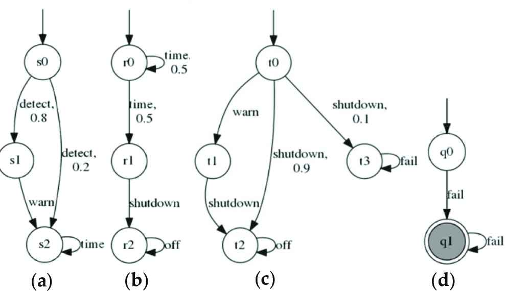
Figure 1 shows two PAs M1 and M2. The switch of a device M2 is controlled by a controller M1. Once the emergence of the detect signal, M1 can send a warn signal before the shutdown signal, but the attempt may be not successful with probability 0.2. M1 issues the shutdown signal directly, this will lead to the occurrence of a mistake in the device M2 with probability 0.1 (i.e., M2 will not shut down correctly). The DFA P err indicates that action fail never occurs. We need to verify whether M1‖M2 ⊨ 〈P〉≥0.98 holds.
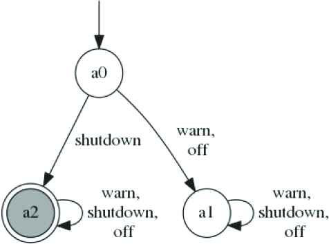
For checking whether 〈true〉M1‖M2 〈P〉≥0.98 holds, we use the rule (SYM) and two probabilistic safety properties 〈AM1〉≥0.9 and 〈AM2〉≥0.8 (see Section 3.2 for details) as the assumptions about M1 and M2. They are represented by DFA
We can compute the probability of AM1 and AM2 in the premise 1 and 2, because we can solve these queries: 〈A〉≥PA M〈P〉IG=? and 〈A〉IA=? M〈P〉≥PG, through multi-objective model checking, as shown in Etessami et al. [18] and Kwiatkowska et al. [33]. Actually, if there exists any adversary of the component M that satisfies the strongest assumption 〈A〉≥1 but violate the probabilistic safety property 〈P〉≥PG, the interval IA will be empty in the second question.
Through premise 3, in
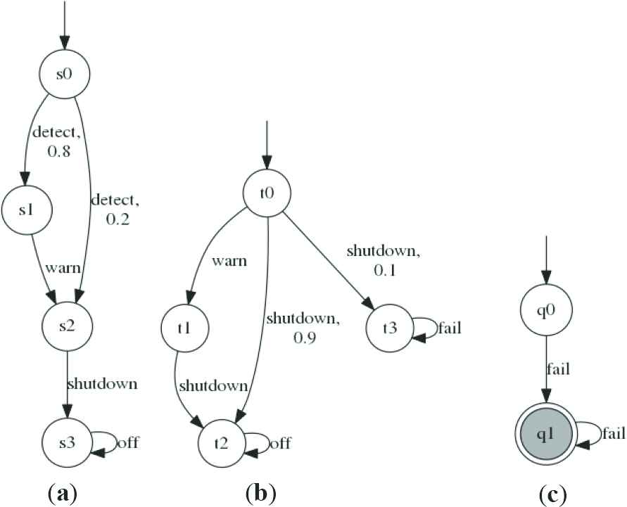
(a) Probabilistic automata M1, (b) probabilistic automata M2 and (c) DFA P err for the safety property P
Assumptions
3.2. Improved Learning Framework for SYM Rule
Inspired by assume-guarantee verification of PAs [23], we propose an improved learning framework that generates assumptions for compositional stochastic model checking two-component PAs with SYM. The inputs are components M1, M2, a probabilistic safety property 〈P〉≥PG and the alphabets αAM1, αAM2. The aim is to verify whether M1‖M2 ⊨ 〈P〉≥PG by learning assumptions. If these assumptions exist, it can conclude that the 〈P〉≥PG holds on the system M1‖M2. It outperforms [23] in cases the model does not satisfy the properties. Essentially, the original learning framework [23] only searches a counterexample after the conjectured assumption generation. Our method is to search a counterexample in each membership and equivalence query to prove M1‖M2 ⊭ 〈P〉≥PG.
3.2.1. Overview
The NL*-based learning framework for compositional stochastic model checking with rule SYM is shown in Figure 3. Here, the MAT first answers a membership query: whether a given finite trace t1 should be included in the assumption AM1. If t1 is not in the assumption AM1, we will try to find corresponding traces in M1 and M2. If their probability violates the probabilistic safety property 〈P〉≥PG, t1 will be not a spurious counterexample. We can think the model does not satisfy the property, otherwise continue to answer the next membership query after checking until the appearance of a conjectured assumption AM1. Then, the MAT answers an equivalence query. Through a multi-objective model checking technique [18,33], we can calculate the probability of a conjectured assumption, which is an interval IA1. If IA1 is an empty interval, the framework will construct a probabilistic counterexample cex(σ, w, c). σ is an adversary for M1 with
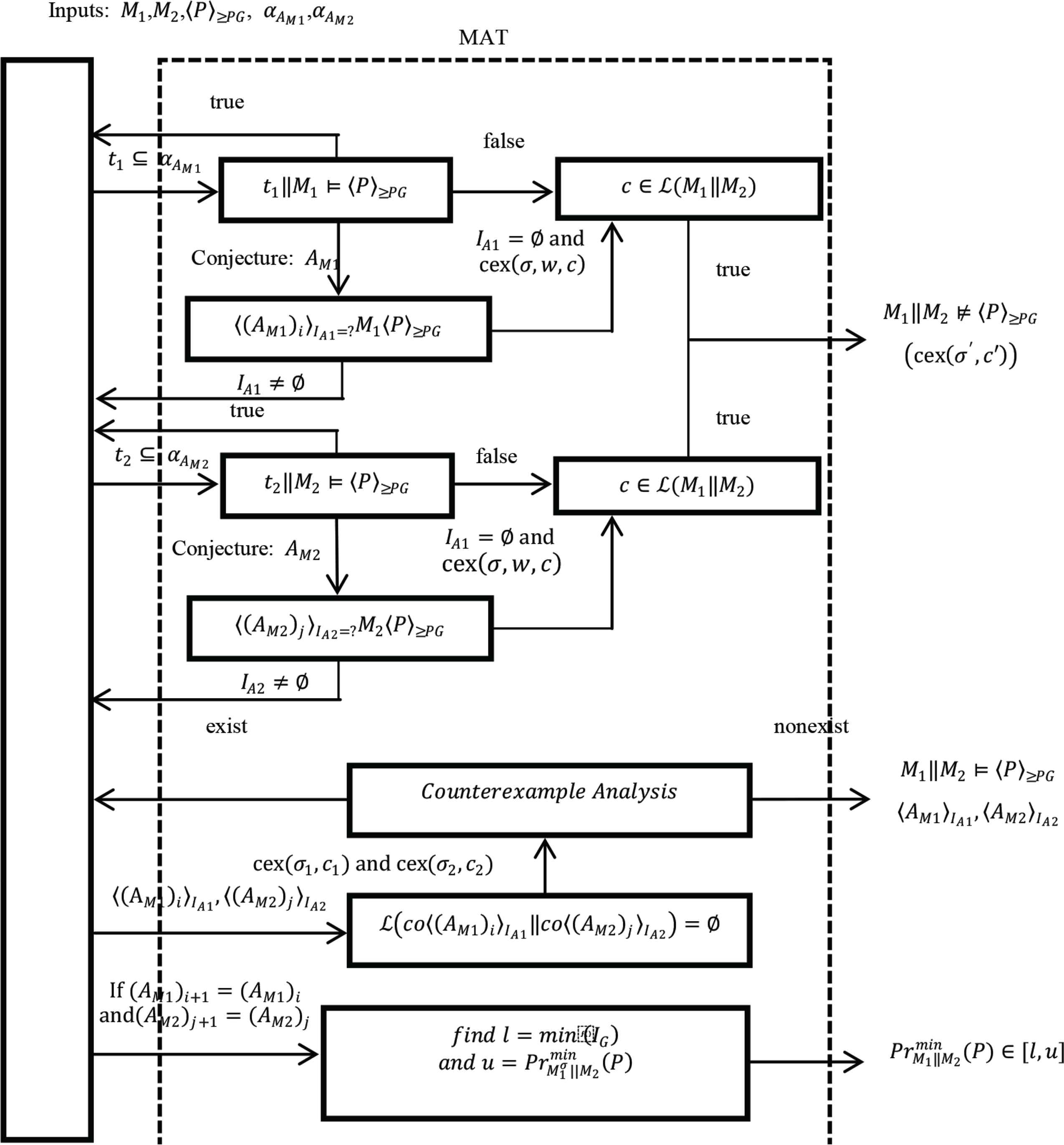
NL*-based learning framework for the rule SYM
On the contrary, we need to check whether it is a spurious counterexample, let the conjectured assumption becomes stronger than necessary. If the spurious counterexample exists, the conjectured assumption must be refined once again. When the conjectured assumption is updated, the framework will return a lower and an upper bound on the minimum probability of safety property P holding. This measure means that it can provide some valuable information to the user, even if the framework could not produce an accurate judgment. More details are described in the following sections.
3.2.2. Answering membership queries
Minimally adequate teacher is responsible for the membership queries, i.e., checking t1‖M1 ⊨ 〈P〉≥PG. t1 represents the trace in which each transition has probability 1. If trace tM1 ∈ M1, tM2 ∈ M2 and tM1↾AM1 = tM2↾AM1 = t1, then P1 and P2 are the probability of trace tM1 and tM2 respectively. If the trace tM1 or tM2 has action fail and P1 * 1 > 1 – PG (i.e., t1‖M1 ⊭ 〈P〉≥PG), t1 will not be included in assumption AM1 and it will be in
Example 2.
We execute the learning algorithm on PAs M1, M2 from Example 1, and the property is set as 〈P〉≥0.99. The alphabet αAM1 is {warn, shutdown, off}, To build its the first conjectured assumption, the algorithm can generate some traces t1:
3.2.3. Answering conjectures for each component
〈(AM1)i〉IA1=? M1〈P〉≥PG (i.e., 〈AM1〉≥PAM1 M1〈P〉≥PG in SYM) can be calculated by multi-objective model checking [18,33]. The widest interval IA1 is defined as [PAM1, 1] and PAM1 = 1 − (1 − PG)/P1. P1 is the probability of trace tM1, if the trace tM1 ∈ M1 or tM2 ∈ M2 has action fail and tM1 ↾AM1 = tM2↾AM1 = t1,
Example 3.
We still execute the learning algorithm on PAs M1, M2 and property 〈P〉≥0.98 from Example 1. The first conjectured assumptions AM1 and AM2 are represented by
tM2 = 〈shutdown, fail〉,
tM2↾AM1 = 〈shutdown〉 = tM1↾AM1,
tM1 = 〈detect, shutdown〉,
PAM1 = 1 − (1 − PG)/P1 = 1 − (1 − 0.98)/0.2 = 0.9.
Similarly, since:
PAM2 = 1 − (1 − PG)/P2 = 1 − (1 − 0.98)/0.1 = 0.8, we can obtain IA2 = [0.8, 1]. We cannot find any trace, which is not in
The first conjectured assumptions
3.2.4. Compositional verification of assumptions
If the interval IA1 and IA2 are nonempty, we will check premise 3 of SYM, we need to verify whether ℒ(co〈(AM1)i〉IA1 ‖ co 〈(AM2)j〉IA2) = Ø. Here, the conjectured assumption AM1 is the one derived after i iterations of learning, similarly for j. PAM1 is the lower bound of the interval IA1, similarly for PAM2.
So ℒ(co〈(AM1)i〉IA1 ‖ co 〈(AM2)j〉IA2) can simplify to ℒ(co〈AM1〉≥PAM1 ‖ co 〈AM2〉≥PAM2), which can convert into the problem whether a prefix of the infinite trace is not accepted by
Finally, if any spurious counterexample trace in
Example 4.
We continue the execution of the algorithm from Example 3. We must do counterexample analysis for it. Intuitively, we can find a spurious counterexample trace cex(0.8, 〈warn, shutdown〉) in
Since 0.8 * 1 = 0.8, we can find that the spurious counterexample trace in
3.2.5. Generation of lower and upper bounds
In each iteration of the NL* algorithm, we can obtain the tightest bounds from the iterative process of assumptions (show in the bottom of Figure 3). If the learning framework cannot provide a definitive result (i.e., the runtime is more than the waiting time), some valuable quantitative information will be returned. For each conjectured assumption, we have a lower bound lb(A, P) and an upper bound ub(A, P) on the probabilistic safety property P.
We can calculate
For the interval
4. ASSUME-GUARANTEE REASONING WITH SYM-N RULE
4.1. Symmetric Rule
We present a symmetric assume-guarantee rule SYM in the previous section, which can solve the problem of verification of a stochastic system about two components. Here, we will make an extension to it. Let it can be used to verify a stochastic system composed of n ≥ 2 components: M1‖M2‖⋯‖Mn.
Theorem 2.
Let M1, M2, …, Mn are PAs, for i ∈{1, 2, …, n}, 〈AMi〉≥PAMi is an assumption for the corresponding component Mi, 〈P〉≥PG is a probabilistic safety property. Their alphabets satisfy αAMi ⊆ αM1 ∪ ⋯ ∪ αMi–1 ∪ αMi+1 ∪ ⋯ ∪ αMn, and αP ⊆ αAM1 ∪ αAM2 ∪ ⋯ ∪ αAMn respectively. co〈AMi〉≥PAMi denotes the co-assumption for Mi which is the complement of 〈AMi〉≥PAMi, the following SYM-N rule holds:
Proof by contradiction.
Assume that the premise 1, 2, …, n + 1 hold, but the conclusion does not. We can obtain an adversary σ ∈ AdvM1‖M2‖⋯‖Mn, such that
Our assumption contradicts (27), so this adversary σ is nonexistent. Next, we will use Example 5 to explain the rule.
Example 5.
The example is the extension of Example 1. Figure 5 shows three PAs M1, M2, M3 and a probabilistic safety property 〈P〉≥0.98. The component M2 indicates that the time signal may reappear with probability 0.5 before the shutdown signal. We will show the verification process by the method of SYM-N rule.
Similar to Example 1, through multi-objective model checking [18,33], we can acquire three assumptions 〈A〉M1 ≥ 0.9, 〈A〉M2 ≥ 1 and 〈A〉M3 ≥ 0.8, which are represented by DFA
Through premise n + 1, we can find a spurious counterexample trace cex(0.2, 〈shutdown〉) in
(a) Probabilistic automata M1, (b) Probabilistic automata M2, (c) Probabilistic automata M3 and (d) DFA P err for the property P

Assumptions
4.2. Improved Learning Framework for SYM-N Rule
The NL*-based learning framework in Figure 7 can be used for verifying a stochastic system composed of n ≥ 2 components: M1‖M2‖⋯‖Mn. We first answer membership queries through solving the problem tj‖Mj ⊨ 〈P〉≥PG, for j ∈ {1, 2, ..., n}. The process is similar to Section 3.2.2 but it is a little different. In Counterexample Analysis for Membership Queries, if tj‖Mj ⊭ 〈P〉≥PG, the framework will verify whether tj is a counterexample c of the target language ℒ(M1‖M2‖⋯‖Mn). If tj is the counterexample c, the framework will return the trace tj and the product of the probabilities of corresponding traces in all components as cex(σ′, c′), and we can find that the property is violated, i.e., M1‖M2‖⋯‖Mn ⊭ 〈P〉≥PG. Then, we need to answer equivalence queries through tackling the problem 〈(AMj)ij〉IAj =? Mj〈P〉≥PG, ij indicates the number of iterations about the assumption AMj and the process of solving the problem shows in Section 3.2.3.
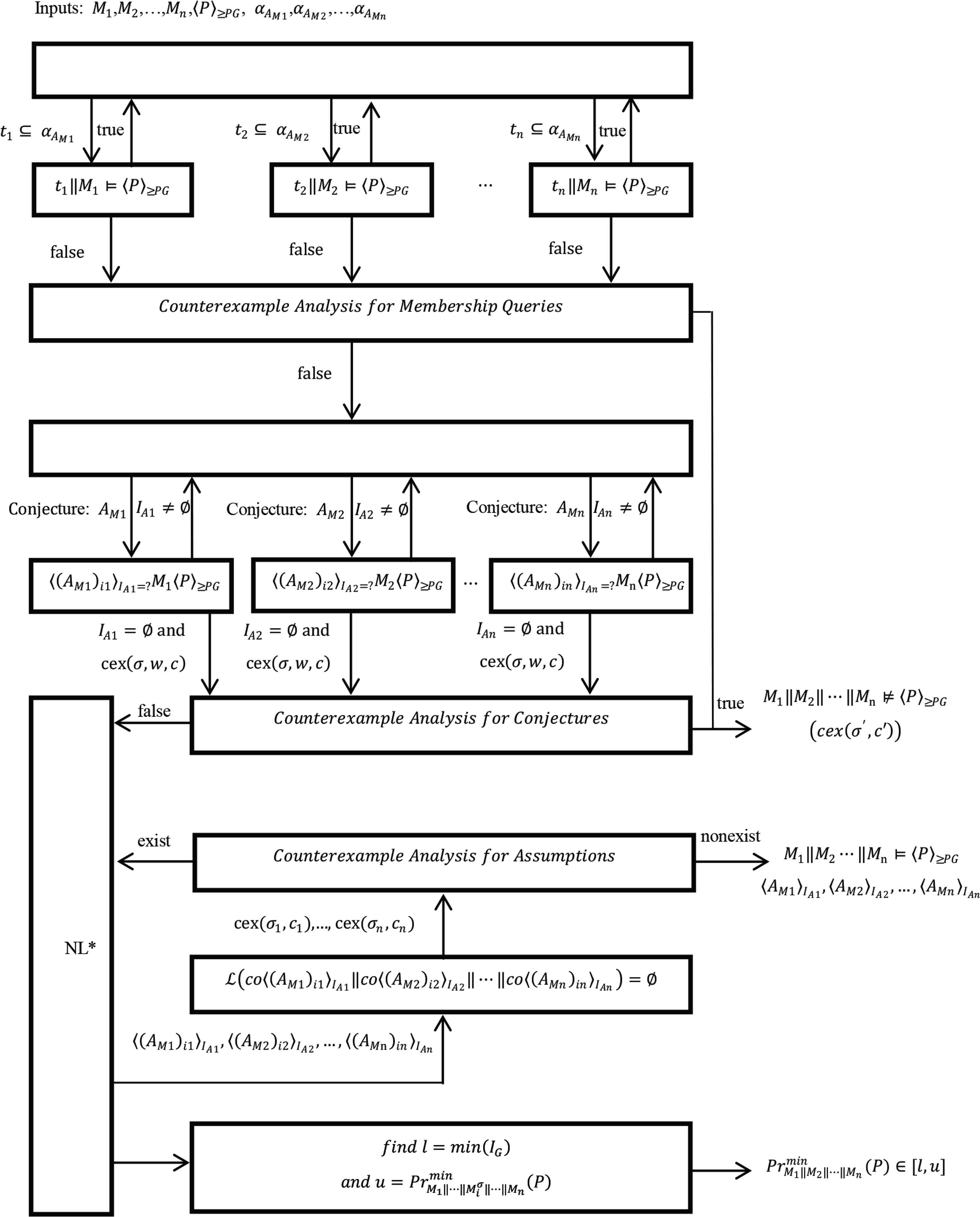
NL*-based learning framework for the rule SYM-N
In Counterexample Analysis for Conjectures, the framework will check if the counterexample cex(σ, w, c) belongs to the target language ℒ(M1‖M2‖ ⋯ ‖Mn). The problem can transform into checking whether
In Counterexample Analysis for Assumptions, if we cannot find any spurious counterexample trace, ℒ(co〈(AM1)i1〉IA1‖co〈(AM2)i2〉IA2‖ ⋯ ‖co〈(AMn)in〉IAn) will be empty and the framework will return assumptions 〈AM1〉IA1, 〈AM2〉IA2, ⋯, 〈AMn〉IAn to prove that the property is satisfied, i. M1‖M2‖⋯‖Mn ⊨ 〈P〉≥PG. On the contrary, we need to use the spurious counterexample traces to weaken the corresponding assumptions. We no longer go into details here.
The framework also can return the tightest bounds of the property P satisfied over the system M1‖M2‖ ⋯ ‖Mn from the iterative process of assumptions. We can calculate:
5. RESULTS
As shown in Figure 8, we have developed a prototype tool for our learning framework. It accepts a model and corresponding property as inputs and returns the verification result. Verification result can be classified into three categories:
- (1)
Some assumptions are provided to prove that model satisfies the property.
- (2)
Counterexample trace cex(σ′, c′) is provided to prove that model violates the property.
- (3)
Bounds of which the property P holds are provided, if the appropriate assumption or counterexample cannot be obtained.
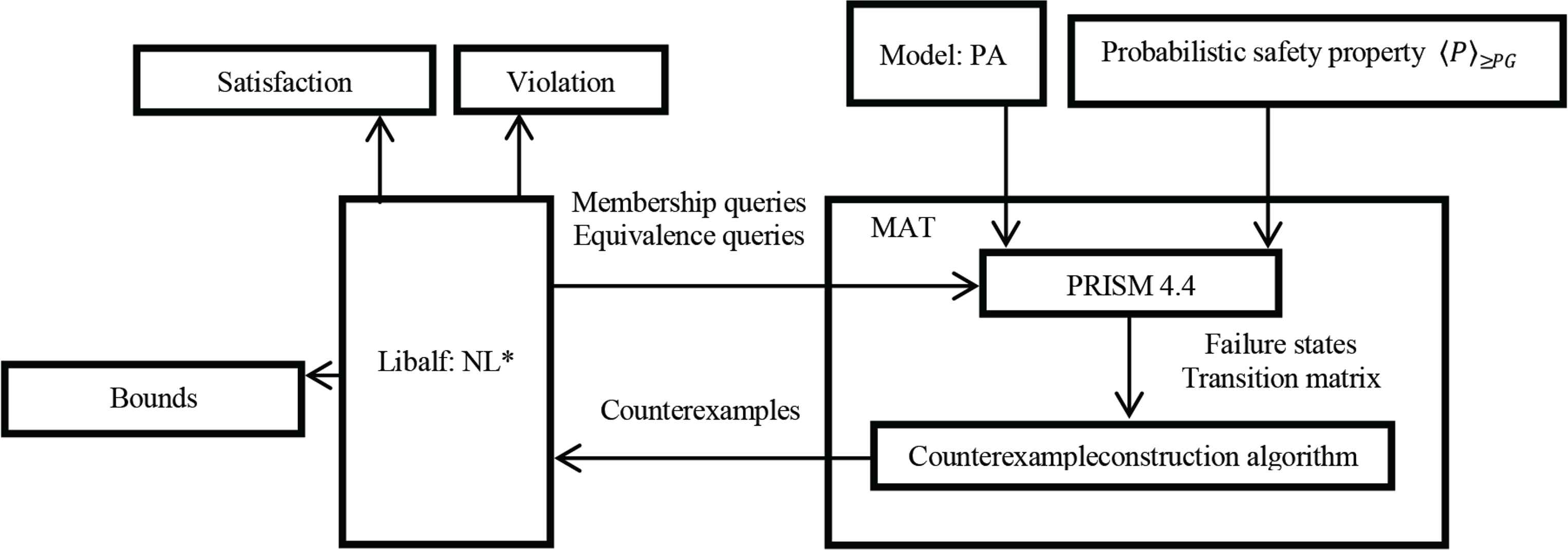
Prototype tool
We use PRISM [25] and counterexample construction algorithm (i.e., particle swarm optimization algorithm [40]) to form a MAT. Then through the libalf [41] learning library, we can implement the NL* algorithm and pose membership and equivalence queries to a MAT. The MAT uses the PRISM modeling language to describe models and probabilistic safety properties. In the interior of the MAT, PRISM can provide the transition matrix (indicate that the transition relation of states in the model) and failure states (indicate that a property is violated) to counterexample construction algorithm. The algorithm can find all shortest paths of the same length and calculate the probability of each path, to construct probabilistic counterexamples. Through constructed counterexamples, we can respond to these queries of libalf. All experiments are run on a 3.3 GHz PC with 8 GB RAM. Feng et al. [22] uses the L* learning algorithm to produce the probabilistic assumptions. On this basis, Feng et al. [23] proves that NL* learning algorithm has more efficient than L* in large-scale cases. Our method thus is based on NL*. We use several large cases to demonstrate our learning framework and compare with the method of Feng et al. [23]. We adopt the first two cases form [23], and modify them a little, because we focus on the conditions that the model does not satisfy the properties. To ensure the correctness of the experimental results, we change the cases through different means. The first case is a network of N sensors. In the network, a channel can issue some data to a processor, but it may crash because some data packets are lost. Through the SYM rule, we make the composition of the N sensors and a channel as a component M1, the processor as the other component M2. We will verify the probabilistic safety property, i.e., network never crashes with a certain probability. We will increase the probability of probabilistic safety property to satisfy our experimental requirements, and the verified property is 〈P〉≥0.994. Table 1 shows experimental results for the sensor network.
| Case study [sensor network] | Sensor numbers | Component sizes | SYM | ASYM [23] | |||
|---|---|---|---|---|---|---|---|
| |M1| | |M2| | MQ | Time(s) | MQ | Time(s) | ||
| 1 | 72 | 32 | 16 | 1.5 | 25 | 2.7 | |
| 2 | 1184 | 32 | 16 | 1.8 | 25 | 2.9 | |
| 3 | 10662 | 32 | 16 | 2.4 | 25 | 3.9 | |
Sensor network experimental results
The second case is the client–server model studied from Pasareanu et al. [42]. Feng et al. [23] injects (probabilistic) failures into one or more of the N clients and changes the model into a stochastic system. In client–server model, each client can send requests for reservations to use a common resource, the server can grant or deny a client’s request, and the model must satisfy the mutual exclusion property (i.e., conflict in using resources between clients) with certain minimum probability. Through the SYM rule, we make the server as a component M1 and the composition of N clients as the other component M2. The verified property is 〈P〉≥0.9.We use the method of Feng et al. [23] to inject (nonprobabilistic and probabilistic) failures into the server respectively. Table 2 shows experimental results for the client–server.
| Case study [client–server] | Client numbers | Component sizes | SYM | ASYM [23] | |||
|---|---|---|---|---|---|---|---|
| |M1| | |M2| | MQ | Time (s) | MQ | Time (s) | ||
| Server (nonprobability) Client (1 failure) | 3 | 16 | 45 | 100 | 2.5 | 161 | 5.2 |
| 5 | 36 | 405 | 325 | 6.9 | 519 | 12.4 | |
| 7 | 64 | 3645 | 833 | 63.1 | 1189 | 140.1 | |
| Server (nonprobability) Client (N failures) | 3 | 16 | 125 | 175 | 4.6 | 213 | 5.9 |
| 4 | 25 | 625 | 336 | 8.3 | 393 | 11.4 | |
| 5 | 36 | 3125 | 226 | 4.9 | 648 | 18.1 | |
| Server (probability) Client (1 failure) | 3 | 16 | 45 | 120 | 0.31 | 187 | 5.7 |
| 5 | 36 | 405 | 379 | 7.8 | 583 | 16.4 | |
| 7 | 64 | 3645 | 937 | 28.1 | 1308 | 45.5 | |
| Server (probability) Client (N failure) | 3 | 16 | 125 | 176 | 3.9 | 265 | 6.6 |
| 4 | 25 | 625 | 337 | 7.4 | 507 | 12.2 | |
| 5 | 36 | 3125 | 568 | 66.2 | 839 | 90.3 | |
Client–server experimental results
To consider the case where the model satisfies the properties, the last case is randomized consensus algorithm from Feng et al. [23] without modification. The algorithm models N distributed processes trying to reach consensus and uses, in each round, a shared coin protocol parameterized by K. The verified property is 〈P〉≥0.97504, and 0.97504 is the minimum probability of consensus being reached within R rounds. Through the SYM rule, the system is decomposed into two PA components: M1 for the coin protocol and M2 for the interleaving of N processes.
In Tables 1 and 2, the component sizes of the M1 and M2 are denoted as |M1| and |M2|, and the performance is measured by the total number of Membership Queries (MQ) and runtimes (Time). Note that Time includes counterexample construction, NFA translation and the learning process. Moreover, for the accuracy of the results, we select the counterexamples in the same order as Feng et al. [23] in each equivalence query. Note that Feng et al. [23] has included comparisons with non-compositional verification, so this paper only compares with Feng et al. [23].
As shown in Tables 1 and 2, the experiment results show that our framework is more efficient than Feng et al. [23]. Obviously, we can observe that, for all cases, runtimes and the number of the membership queries in our framework are less than Feng et al. [23]. Moreover, the runtimes need less in our framework, when the model has a large scale. A larger size model may have less runtimes and the number of membership queries than a smaller model. However, this is not proportion with the model size. The efficiency of our framework depends only on the time of a counterexample (indicate that the probabilistic safety property is violated) appears in conjectured assumptions. The earlier a counterexample appears, the more efficient our framework performs.
In Table 3, the component sizes of the M1 and M2 is also denoted as |M1| and |M2|. The performance is measured only by total runtimes (Time), because both methods have the same amount of MQ if the model satisfies the properties. Because of the cost of early detection, we can find that our methods need to spend more time than Feng et al. [23] and cost grows with the model size. But compared with acquirement of optimization in Tables 1 and 2, the cost is acceptable in Table 3.
| Case study [consensus] | [N R K] | Component sizes | SYM | ASYM [23] | |
|---|---|---|---|---|---|
| |M1| | |M2| | Time (s) | Time (s) | ||
| 2 3 20 | 3217 | 389 | 12.1 | 11.6 | |
| 2 4 4 | 431649 | 571 | 82.2 | 80.7 | |
| 3 3 20 | 38193 | 8837 | 355.8 | 350.2 | |
Randomized consensus algorithm experimental results
Table 4 compares the performance of the rule (SYM) and the rule (SYM-N). We impose a time-out of 5 h. Sensor network model has N sensors and client–server model has N clients. In client–server model, each client and server all have a (probabilistic) failure. For the use of rule (SYM-N), we decompose M1 into separate sensor and compose each sensor and a channel as a component in sensor network model, and decompose M2 further into separate client in client–server model. Moreover, the performance is measured by the total runtimes (Time). In all large cases, the rule (SYM-N) has more advantage than the rule (SYM). For example, in the case of sensor network model with four sensors, the component M1 has 72776 states and the component M2 has 32 states. The total runtime of the compositional verification by the rule (SYM) more than 5 h, but the use of the rule (SYM-N) only needs 16.6 s. This is because the size of the component M1 is too large for the rule (SYM), and the counterexample construction algorithm needs more time to give the conclusion.
| Case study [parameters] | Component sizes | SYM | SYM-N | ||
|---|---|---|---|---|---|
| |M1| | |M2| | Time (s) | Time (s) | ||
| Sensor network [N] | 4 | 72776 | 32 | Time-out | 16.6 |
| 5 | 428335 | 32 | Time-out | 40.7 | |
| Client–server [N] | 6 | 49 | 15625 | Time-out | 20.4 |
| 7 | 64 | 78125 | Time-out | 80.9 | |
Performance comparison of the rule (SYM) and the rule (SYM-N)
6. DISCUSSION
We first present a sound SYM for compositional stochastic model checking. Then, we propose a learning framework for compositional stochastic model checking PAs with rule SYM, based on the optimization of LAGR techniques. Our optimization can terminate the learning process in advance, if a counterexample appears in any membership and equivalence query. We also extend the framework to support the assume-guarantee rule SYM-N which can be used for reasoning about a stochastic system composed of n ≥ 2 components: M1‖M2‖ ⋯ ‖Mn. Experimental results show that our method can improve the efficiency of the original learning framework [23]. Similar to Feng et al. [22] and Kwiatkowska et al. [33], it can return the tightest bounds for the safety property as a reference as well.
In the future, we intend to develop our learning framework to produce richer classes of probabilistic assumption (for example weighted automata as assumptions [39]) and extend it to deal with more expressive types of probabilistic models.
CONFLICTS OF INTEREST
The author declare they have no conflicts of interest.
ACKNOWLEDGMENTS
This work was supported by the
REFERENCES
Cite this article
TY  - JOUR
AU  - Yang Liu
AU  - Rui Li
PY  - 2020
DA  - 2020/04/09
TI  - Compositional Stochastic Model Checking Probabilistic Automata via Assume-guarantee Reasoning
JO  - International Journal of Networked and Distributed Computing
SP  - 94
EP  - 107
VL  - 8
IS  - 2
SN  - 2211-7946
UR  - https://doi.org/10.2991/ijndc.k.190918.001
DO  - 10.2991/ijndc.k.190918.001
ID  - Liu2020
ER  -