
Improvement of CSF, WM and GM Tissue Segmentation by Hybrid Fuzzy – Possibilistic Clustering Model based on Genetic Optimization Case Study on Brain Tissues of Patients with Alzheimer’s Disease
- DOI
- 10.2991/ijndc.2018.6.2.2How to use a DOI?
- Keywords
- Fuzzy c-means algorithm; Possibilistic c-means algorithm; Genetic algorithms; Hybrid reasoning; Brain tissue clustering; Alzheimer’s disease
- Abstract
Brain tissue segmentation is one of the most important parts of clinical diagnostic tools. Fuzzy C-mean (FCM) is one of the most popular clustering based segmentation methods. However FCM does not robust against noise and artifacts such as partial volume effect (PVE) and inhomogeneity. In this paper, a new approach for robust brain tissue segmentation is described. The proposed method quantifies the volumes of white matter (WM), gray matter (GM) and cerebrospinal fluid(CSF) tissues using hybrid clustering process which based on: (1) FCM algorithm to get the initial center partition. (2) Genetic algorithms (GA) to achieve optimization and to determine the appropriate cluster centers and the fuzzy corresponding partition matrix. (3) Possibilistic C-Means (PCM) algorithm for volumetric measurements of WM, GM, and CSF brain tissues. (4) Rule of the possibility maximum to compute the labeled image in decision step. The experiments were realized using different real and synthetic brain images from patients with Alzheimer’s disease. We used Tanimoto coefficient, sensitivity and specificity validity indexes to validate the proposed hybrid approach and we compared the performance with several competing methods namely FCM and PCM algorithms. Good result was achieved which demonstrates the efficiency of proposed clustering approach and that it can outperforms competing methods especially in the presence of PVE and when the noise and spatial intensity inhomogeneity are high.
- Copyright
- Copyright © 2018, the Authors. Published by Atlantis Press.
- Open Access
- This is an open access article under the CC BY-NC license (http://creativecommons.org/licences/by-nc/4.0/).
1. Introduction
The classification of brain tissues including the quantification of tissue volumes are a necessary step in many medical imaging applications. The resulting segmentation yields a patient-specific demarcation of individual tissues. This permits the quantitative characterization of the tissues and the construction of patient specific models of tissue conductivity [1].
Moreover, regional volume calculations may bring even more useful diagnostic information. Among them, the quantization of grey matter (GM), white matter (WM) and cerebrospinal fluid (CSF) tissues volumes would be most useful for diagnosis and treatment of pathologies, and may be of major interest in neurodegenerative disorders such as Alzheimer disease (AD), Parkinson related syndrome, in WM metabolic or inflammatory disease, in congenital brain malformations or perinatal brain damage, or in post-traumatic syndrome [2].
However, the tissue volumes quantification is one of the most challenging tasks in image processing for many reasons, some of which are [3,4,5,6]: (1) medical images contain inherent constraints that make the resulting image noisy and may include or introduce some visual artefacts such as partial volume effects (PVE) and spatial inhomogeneity. (2) Image data can be ambiguous and susceptible to noise and high frequency distortion, where object edges become fuzzy and ill-defined.
Indeed, the brain image segmentation is a complex and challenging task due to errors in the scanner resulting from inhomogeneities in the magnetic field and biological variations between subjects. Other generating factors are to be expected such as the inherently imprecise nature of the images in calculations, the vagueness in class definitions and expert knowledge [7], and the uncertainty of some of sources which contain additive and non-additive noise. Therefore, every voxel is influenced by the PVE and belonging to different brain tissues. Unfortunately, this limits the overall diagnostic potential in the clinical context.
To fix this problem, several authors [8,9,10,11,12] have reviewed some image segmentation techniques using pattern recognition, making a distinction between on the one hand, supervised methods [13,14,15,16] with modeling of the image by Markov or Gibbs random field, Bayes’ classifier with estimation by maximum likelihood expectation, k nearest neighbors. On the other hand, unsupervised algorithms [17,18,19,] with hard [14,20] and fuzzy [21,22,23,24] clustering techniques.
Fuzzy based image clustering techniques are widely used due to effective segmentation performance. Clustering is a process that allows dividing data into groups of similar pattern called clusters [25]. In the literature, there are several fuzzy clustering techniques. Nothing that the first notion of fuzzy theory was proposed by Zadeh [26] who established the basic principle of fuzzy theory using the fuzzy logic, in order to describe the uncertainty of belonging by a membership function. Then Ruspini [27] proposed the first notion of a fuzzy partition who considers that each cluster is a fuzzy set. After, Zadeh [28] proposed the conceptual framework for cluster analysis and pattern classification using the fuzzy set theory. Later, several researches were published in order to improve the Bezdek algorithm [29] and to make fuzzy c-means (FCM) algorithm robust against noise and artifacts such as PVE and inhomogeneity.
Traditionally, probability theory was the primary mathematical model used to deal with uncertainty problems [9] however, the possibility concept introduced by the fuzzy set theory has gained popularity in modeling and propagating uncertainty in imaging applications [30]. The membership values generated by FCM using the FCM constraint ( eq. 3 ) represent the degree of sharing, but not the degree of typicality or compatibility with an elastic constraint. Typicality here means the actual degree of belongingness of a datum to a cluster rather than an arbitrary division of data [31, 32, 33]. Krishnapuram et al. [32] addressed these issues by proposing the possibilistic c-means (PCM) algorithm whose membership values represent the degree of typicality rather than the degree of sharing and as consequence constraint ( eq. 3 ) is eliminated [32, 34]. Every cluster is independent of the other clusters in PCM algorithm.
The aim of this paper is to evaluate the effectiveness of possibilistic theory which managing uncertainty and imprecision. We choose then the PCM algorithm for volumetric measurements of WM, GM and CSF brain tissues. We used then PCM algorithm to create fuzzy tissue maps of brain images instead FCM and its variations because, this possibilistic algorithm allows to interpret memberships as absolute degrees of belonging whereas, they are similar to degrees of sharing in the case of FCM or extensions. Moreover, the PCM algorithm is more robust in the noisy environment then FCM algorithm.
Moreover, we propose a genetic – fuzzy process for centers initialization of PCM clusters. For this purpose, we use the FCM algorithm [11, 35] to get the initial partition and genetic algorithms (GA) [36] to achieve optimization and choose at the end of accounts the best score among all. The integration of genetic process is to determine the appropriate cluster centers and the fuzzy corresponding partition matrix. This initialization process allows us to train the possibilistic algorithm with centers partition obtained with empiricism and not by the random which avoids local minima and it allows the process to converge quickly.
Clustering results are reported for several simulated T1-weighted, Magnetic Resonance (MR), Single Photon Emission Computed Tomography (SPECT) and Positron Emission Tomography (PET) brain images belonging to patients suffering from AD. These images obtained from synthetic ADNI (Alzheimer’s Disease Neuroimaging Initiative ) phantom [37] and from Gabriel Mont pied hospital real database [38]. Superiority of the proposed method over both conventional FCM and PCM algorithms are demonstrated.
The paper is organized as follows: Section 2 deals with literature survey in medical imaging field. Section 3 explains the principle of the hybrid clustering process used for quantization of different tissue classes. Sections 4 and 5 present the implementation and results for clinical case of AD. Finally, section 6 concludes and discusses this work.
2. Related-work
There are huge amount of works related to enhancing the conventional FCM for image segmentation which are found in the literature and that are proposed for increasing the robustness of FCM against PVE and noise.
In [39], the FCM distance-based algorithm has been generalized into the Evidential C-Means algorithm (ECM) [40], which allows representing ambiguous information in the feature space on disjunctions in an unsupervised way.
The authors in [41] have presented an approach for improving range image segmentation based on fuzzy regularization of the detected edges. The segmentation process was repeated for all region boundaries in the image using an improved version of the FCM algorithm.
To deal with intensity in homogenities, the authors in [11] proposed an adaptive FCM. In this case, the centroids are multiplied by unknown multiplier filed, which represents the inhomogeneity. First and second order regularization terms are included in the cost function to make the multiplier field varying slowly and smoothly.
Pham and Prince [42,43] proposed an Adaptive FCM algorithm (AFCM) that produces a soft segmentation while simultaneously adapting to intensity inhomogeneities in the image. The algorithm was derived by incorporating a gain field term into the objective function of the standard FCM algorithm. While AFCM has been shown to be effective in correcting for inhomogeneities, its main disadvantage is that its performance degrades significantly with increased noise.
In Karan Sikka et al. [44], a fully automated brain MR image segmentation algorithm under modified FCM framework is proposed. An entropy driven homomorphic filter is used for in-homogeneity correction. A method namely histogram-based local peak merger using adaptive window is proposed to initialize cluster centers. The results of the algorithms are compared quantitatively to investigate their effectiveness in classification of GM, WM and CSF tissues.
A two-dimensional FCM (2DFCM) algorithm was proposed in [45] for the molecular image segmentation. The three steps of the algorithm are: noise suppression, texture energy characterization, and introducing spatial constraints into the fuzzy clustering. The segmentation results are satisfactory for the images corrupted by noise and intensity variations.
In [29,35], the authors used multidimensional features formed by GLCM (Grey Level Co-occurrence Matrix) feature generation model to include spatial information into FCM. Extra dimensions make the process time consuming so to overcome this, distance metric based compression is proposed to select the representative pixels of the groups and perform clustering on them, which resulted in fast and effective clustering.
A high speed parallel FCM algorithm for brain tumor image segmentation is presented in [46]. Their algorithm has the advantages of both the sequential FCM and parallel FCM for the clustering process in the segmentation techniques and the algorithm was very fast when the image size was large.
The work presented in [47] deals with brain MRI segmentation. The distinct regions are represented by wavelet coefficients. Classification of these features was performed using FCM algorithm. Edge detection technique was used to detect the edges of the given images. Silhouette method was used to find the strength of clusters.
In [48], Gaussian smoothing was performed on input image proposing a method to find the weightage for each feature using bootstrapping technique when dealing with multiple features.
Improved FCM (IFCM) to deal with noise affect is proposed in [49]. In IFCM the distance term of FCM is modified by including two terms, feature attraction and distance attraction.
A prior probability and fuzzy spatial information are used in ISFCM (Improved Spatial FCM) algorithm, proposed in [50] to minimize the noise affect in MRI images. In the study, cluster centers are initialized using histogram based FCM.
In [51], a novel fuzzy energy minimization method was presented for simultaneous segmentation and bias field estimation of medical images.
In [52], the effectiveness of the FCM algorithm in terms of computational rate is improved by modifying the cluster center and membership value updating criterion.
In [53], the comparison of the three fundamental image segmentation methods based on FCM, Intuitionistic FCM (IFCM), and Type-II FCM (T2FCM) is presented. These algorithms are executed in two scenarios– both in the absence and in the presence of noise and on two kinds of images– Bacteria and CT scan brain image.
In [54], a Picture Fuzzy Clustering (PFC) method was presented for MRI brain image segmentation. The PFC is based on the picture fuzzy set, which is the generalization of the traditional fuzzy set and intuitionistic fuzzy set.
In [55], the application of modified FCM algorithm for MR brain tumor detection is explored. A comprehensive feature vector space is used for the segmentation technique.
Although FCM and its variants are a very useful clustering methods, its memberships do not always correspond well to the degrees of belonging of the data, and they may be inaccurate in a noisy environment [32]. In another sense, the FCM algorithm and its extensions create relative memberships interpreted as degrees of sharing of the voxels between all the classes, that are thus unrepresentative of the true degree of belonging.
3. Principle of possibilistic clustering based on fuzzy-genetic initialization
Fig. 1. schematizes the proposed classification process. This process is composed of three-step of segmentation:
- •
Cluster centers initialization with FCM/GA process and which is necessary for subsequently applying the PCM algorithm.
- •
Image modeling, for which the fuzzy tissue maps are created using PCM algorithm and the information extracted from the images is modeled in a common theoretical frame.
- •
Image labeling, which synthesizes the available information by creating a labeled image.
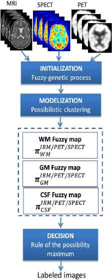
Proposed general scheme for tissue quantification.
3.1. Cluster center initialization
We applied FCM to determine the appropriate cluster centers bi and the corresponding fuzzy partition matrix U of PCM algorithm.
The FCM clustering uses iterative optimization to approximate minima of a constrained objective function [9]:
Where N is the number of voxels that need to be partitioned into C tissues, uij is the membership function of the element xj (a feature vector at position j) belonging to the ith cluster, m is the weighting exponent that controls the fuzziness of the resulting partition (most often is set to m = 2) and d(xj, bi) is the similarity measure between xj and the ith cluster center bi. The most commonly used similarity measure is the squared Euclidean distance:
The objective function JFCM ( equation (1) ) is minimized under the following constraints:
Considering these constraints, the membership degrees uij and clusters centers bi are given as follows:
The FCM algorithm iteratively optimizes JFCM, by evaluating (4) and (5) , until the following stop criterion is satisfied:
The FCM algorithm is composed of the following steps:
| FCM steps |
|---|
Let X = {xj/j = {1 … N}} the voxels set, U = (uij)1≤i≤C,1≤j≤N the matrix of membership degrees, B = (bij)1≤i≤C,1≤j≤N the matrix of cluster centers, m the degree of fuzzy and ε the threshold representing convergence error.
|
We applied FCM algorithm to determine the appropriate centroids bi of clusters before optimization with GA.
3.2. Optimization of FCM results with GA
The result of FCM clustering was used as initial population for GA. This allows training the GA with a population of empirically generated chromosomes and not randomly initialized.
The GA started with a population composed of the set of FCM results which represent the fuzzy corresponding partition matrix. Solutions from one population are taken and used to form a new population. This is motivated by a hope, that the new population will be better than the old one. Solutions which are selected to form new solutions (offspring) are selected according to their fitness - the more suitable they are the more chances they have to reproduce.
The following merit function was used to assess the fitness of a chromosome [36]:
The crossover and mutation are the most important part of the GA. The performance is influenced mainly by these two operators. Crossover selects genes from parent chromosomes and creates a new offspring. After a crossover is performed, mutation take place. This is to prevent falling all solutions in population into a local optimum of solved problem. Mutation changes randomly the new offspring.
The strong points is that GA are intrinsically parallel, easily distributed and the concept are easy to understand. Nothing also that the optimization required less time and chances of getting optimal solution are more. The initialization with hybrid FCM-GA approach avoids local minima and allows the PCM clustering based image modelling to converge quickly.
3.3. Image modeling with PCM algorithm
Although FCM is a very useful fuzzy clustering method, its memberships do not always correspond well to the degree of belonging of the data, and may be inaccurate in a noisy environment [3]. To improve this weakness and to produce memberships that have a good explanation for the degree of belonging, Krishnapuram and Keller [32] relaxed the constrained condition
The PCM algorithm assigns typicality values to fuzzy membership functions [32]. Thus in PCM, the elements of the partition matrix, denoted by tij instead of uij (i = 1…C, j = 1…N), describe how compatible the input vectors are with the clusters represented by the computed cluster prototypes. Typicality values with respect to one cluster do not depend on any of the prototypes of other clusters.
In our case, PCM algorithm gives a set of three fuzzy maps corresponding to WM, GM, and CSF tissues which are fuzzy and absolute, and allows to compute the degree of membership of each voxel to brain tissue. Nothing that these voxels are characterized by a feature vector composed of its gray levels in the different images.
PCM associates with every feature vector xj, a typicality degree tij ∈ [0, 1] in each of the C clusters, representing the degree that has xj to belong to i. In the PCM algorithm, each cluster is independent of the other clusters. Iterative optimization is used to approximate minima of a constrained objective function JPCM corresponding to cluster i. JPCM can be formulated as [57]:
The PCM algorithm is composed of the following steps:
| PCM steps |
|---|
The entries
|
| Step1 Initialize the the centers vectors B(0)=[bj] using FCM-GA method. |
| Step2 At k-step: |
| Step3 Update: B(k+1) and T(k+1) |
| Step4 If ‖J(k+1) − J(k)‖ < ε then STOP otherwise return to step 2. |
The stopping criterion defines the stability or the convergence of the process. In most cases, it represents the stability of the clusters centers by successively iterating the steps 2 and 3.
Krishnapuram and Keller [32], and Barra [38] proved that the PCM membership of a vector xj to class i only depends on xj and i and not on the memberships of xj in all other classes (as is the case for FCM). This is very convenient in the case of strong ambiguity or uncertainty, which can occur in scan images (PVE, noise), as shown by clear examples in Krishnapuram and Keller [32].
We clustered all images with PCM algorithm, thus obtaining three sets of fuzzy maps: (WMMRI, GMMRI, CSFMRI), (WMPET, GMPET, CSFPET), and (WMSPECT, GMSPECT, CSFSPECT). These maps are related to three distributions of possibility
Information of images is now represented in a common theoretical frame (distributions of possibility), and the result can now be used in the segmentation step to obtain the labeled image.
3.4. Image labeling process
After applying PCM modeling for each image, the degrees of possibility provided will be exploited for image labeling and a segmented image was finally computed using the three fuzzy maps obtained in the previous step.
Each voxel v is assigned to label tissue {GM, WM, CSF} which corresponds to the highest degree of possibility in {πGM(ν), πWM(ν), πCSF(ν)} as follow:
4. Experiment on patients with Alzheimer’s disease
The objective of this study is to cluster registered MR, PET and SPECT brain images corresponding to patients suffering from AD according to the neuro-psychological assessment. A simple definition of these three types of scans is as follows:
A MR scan uses a strong magnetic field and radio waves to create a detailed cross-sectional images of the patient’s internal organs and tissues within the body.
A PET scan uses radioactive tracers to produce 3-D, color images of the inside of the human body. It can measure blood flow, oxygen use, glucose metabolism, and much more.
A SPECT scan is a type of nuclear imaging test, which means it uses a radioactive substance and a special gamma camera to create 3-D pictures. It can show how blood flows to the heart or which areas of the brain are more active or less active.
4.1. Information on participants
4.1.1. Synthetic brain data
PET and MR Data used to prepare this work were obtained from the ADNI phantom site1. The ADNI was launched in 2003 by the National Institute on Aging, the National Institute of Biomedical Imaging and Bioengineering, the Food and Drug Administration, private pharmaceutical companies and nonprofit organizations, as a $60 million, 5-year public-private partnership [37].
We used 45 AD subjects between 55 and 90 years of age with all corresponding baseline MR and PET images are included.
4.1.2. Real brain data
The real images set that is available to validate tissue quantification approaches is a protocol developed at the Gabriel Mont pied Hospital in Clermont-Ferrand (France) [38]. We used MR, PET and SPECT scans that concern five patients (three men and two women) aged 71–86 years suffering from AD.
The simulated models consisted of a set of 3D fuzzy tissue membership volumes, one for each tissue class (WM, GM and CSF).
4.2. Imaging Parameters
4.2.1. ADNI data acquisition
A detailed description of MR and PET protocols and acquisition is as follows:
MRI – All subjects were scanned with a standardized high-resolution MRI protocol on scanners developed by one of three manufacturers (General Electric Healthcare, Siemens Medical Solutions and Philips Medical Systems) with a protocol optimized for best contrast to noise in a feasible acquisition time [37]. Raw Digital Imaging and Communications in Medicine (DICOM) MRI scans were downloaded from the public ADNI site1. The MR volume has 256 × 256× 176 voxels covering the whole brain and yielding a 1.0 mm isotropic resolution.
PET – All the baseline PET data was downloaded from the ADNI web site1. PET images were acquired 30–60 min post-injection, averaged, spatially aligned, interpolated to a standard voxel size, intensity normalized and smoothed to a common resolution of 8-mm full width at half maximum [58]. The reconstructed images had a matrix size of 256 × 256 × 207 voxels with a voxel size of 1.2 × 1.2 × 1.2 mm3.
4.2.2. Gabriel Mont pied Hospital data acquisition
For MR image acquisition, the T1-weighted rapid gradient echo sequence (TR = 2600 ms and TE = 3.0 ms) was selected. The slice thickness of the images is 1 mm with no space considered between the slices. The MR volume has 256 × 256 × 176 voxels which covers the whole brain with an isotropic resolution of 1.0 mm.
To obtain the PET images, each patient received two successive scans, the first is of transmission which lasted 6 minutes, and the second is of emission of 20 minutes which was started after the injection of 555 Mq of [11C]-PIB. The size of the reconstructed images is 256 × 256 × 207 voxels with a voxel size of 1.2 × 1.2 × 1.2 mm3.
For SPECT images, an injection of 25 mCi (9.25 3 108 Bq) of Tc-99mHMPAO was made. The acquisition of the images was then carried out after 10 minutes on a SOPHA DSX camera using a high-resolution parallel low-energy collimator. Sixty-four projections were recorded for 30 s each. Sixty-four slices of size 64 × 3 × 64 were then reconstructed using filtered back-projection with a Butterworth filter (cutoff frequency 0.25).
4.3. Preprocessing
First we developed an image of multiple regions where the gray level inside each region varies within certain limits. Then we added white Gaussian noise with different signal to noise ratio (SNR). A hybrid median filter was applied on the images. Several images of the same brain were created with 1% to 7 % of additive noise, with slice thickness ST (1 mm) and their radiofrequency (RF) inhomogeneity is 20% intensity non-uniformity).
4.4. Center initialization process for PCM modelling
The FCM-GA clustering process is applied to a brain slices to get the cluster centers. The result of FCM clustering was used as initial population for GA. After application of FCM, the gray level of each voxel in the volumes reflected the proportion of tissue present in that voxel. So, GA based clustering algorithm are executed for 20 generations with fixed FCM population size 15. The crossover and mutation probabilities are fixed as Pc = 0.8 and Pm = 0.01, respectively. These values are chosen after many experiments. After convergence generation with the lowest fitness value [36], we choose the obtained centers to start the modeling by PCM.
4.5. Tissue possibilistic modeling
We clustered the brain images with PCM algorithm for which FCM-AG process has been used for centers initialization. The result obtained from the execution of the PCM algorithm to the image k ∈ {1..P} is a series of three fuzzy maps corresponding to the tissue T∈ {CSF, GM, WM} estimated from the image k, (see Fig. 2). In this figure and in each map, the WM, GM and CSF tissues are expressed by the zones with white color.
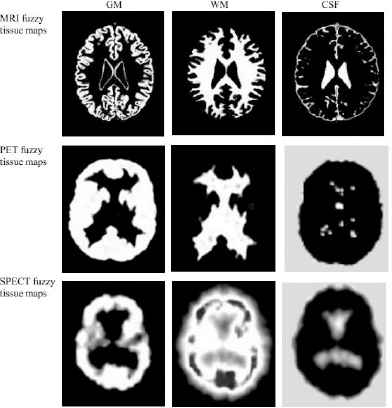
Computed fuzzy tissue maps derived from a MR, SPECT and PET images slices.
For the parameter m which controls the degree of fuzziness of the resulting fuzzy maps; if m is close to 1, the partition generated by PCM is almost crisp, and memberships become fuzzier as m increases. When m tends to infinity. All the memberships for a given voxel are equal to 1/C. There is no optimization process to compute the “best” m, it greatly depends on the nature of the data. We follow the suggestions proposed in [59] and we propose finding m in [1.5, 5], which gives the “best” partition of our brain images. Then, we have trained the algorithm with values in the interval [1.5, 5]. After some experimentation, we chose m = 2 with the application of a Euclidean distance and a threshold of convergence, ε = 0.005.
The images Information is now represented with distributions of possibility, so it is expressed in a common theoretical frame. Then the result could be used in the final segmentation step.
4.6. Final segmentation
A labeled image, created by assigning each voxel to the tissue class, for which it had the greatest membership. An example of both reference and computed segmented images are presented in Fig. 3. Nothing that the ground truth information is available from the synthetic and real databases.
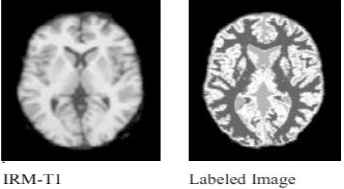
Example of labeled image of a real IRM-T1 image slice. Tissues are labeled WM (dark gray color), GM (white color), and CSF (gray color).
5. Comparative performance
The performance of the proposed clustering method have been compared with some other widely used clustering algorithms viz., the conventional FCM and PCM algorithms.
5.1. Methods
For comparing the performance some validity measures, are considered. These are defined below.
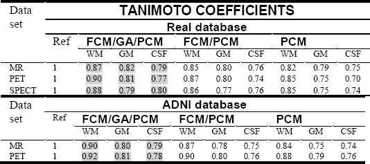
5.1.1. Tanimoto coefficient (TC)
It was defined for a given tissue in computed and ground truth segmentation as the number of voxels that had a good tissue assignment in computed segmentation divided by the sum of voxels of tissue assignment in ground truth segmentation. It is close to 1 for very similar results and is near 0 when the labeled images share no similarly classified voxels [60].
5.1.2. Sensitivity (SE)
It corresponds to the proportion of true positives (TP) compared to all of the voxels that should be segmented.
In our application, this indicator allows determining the percentage of voxels that are correctly identified as belonging to the tissue in question. SE tends to 1 (resp. 0) if there is little (resp. much) of false negatives (FN).
5.1.3. Specificity (SP)
It corresponds to the proportion of true negatives (TN) compared to all of the voxels that should not be segmented:
In our application, this indicator allows determining the percentage of voxels that are properly identified as belonging to complementary tissues. SP tends to 1 (resp. 0) if there is little (resp. a lot) of false positives (FP).
5.2. Experimental Result
Table 1., Table 2. and Table 3. report the Tanimoto coefficients, sensitivity and specificity values with RF inhomogeneity = 20 %, slice thickness = 1 mm and 1% to 7% of SNR, for all tissues and for different clustering algorithms used in this experience. We plotted also in Fig. 4., Fig. 5. and Fig. 6. the curves of sensitivity and specificity clustering indexes with SNR varying between 1% to 7% for visualizing the results.
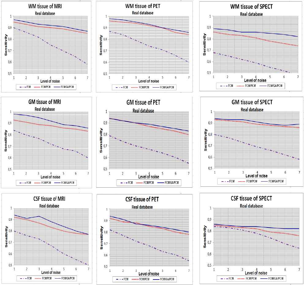
Curves of sensitivity clustering index for WM, GM and CSF tissue with 1%…7% SNR, using FCM, FCM/PCM and FCM/GA/PCM clustering algorithms, application for real database.
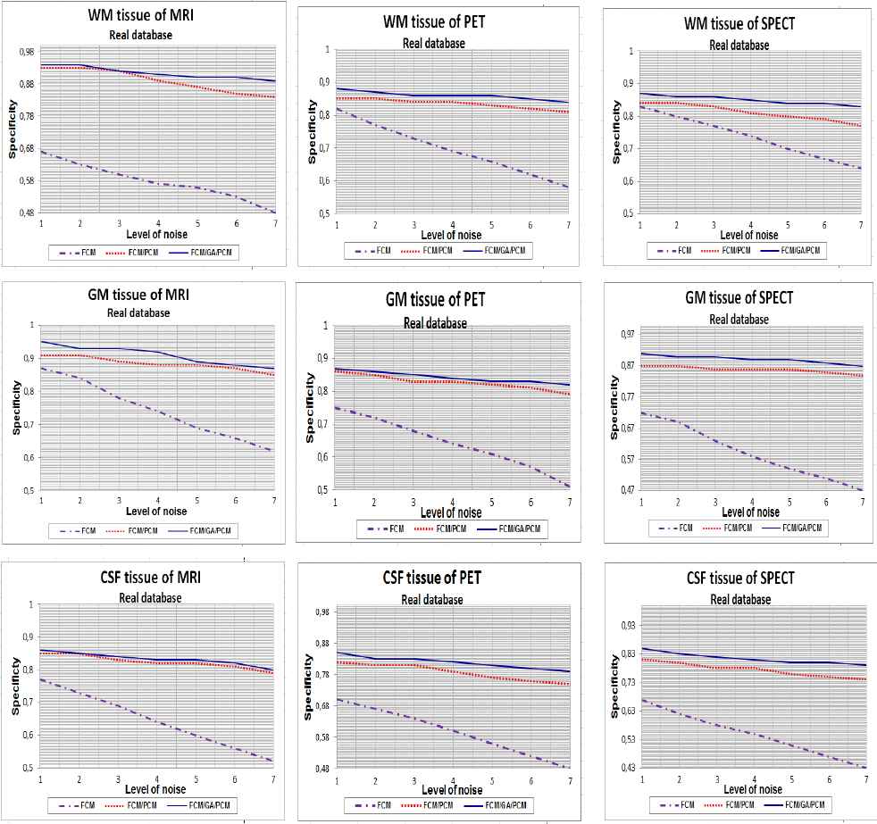
Curves of specificity clustering index for WM, GM and CSF tissue with 1%…7% SNR, using FCM, FCM/PCM and FCM/GA/PCM clustering algorithms, application for real database.
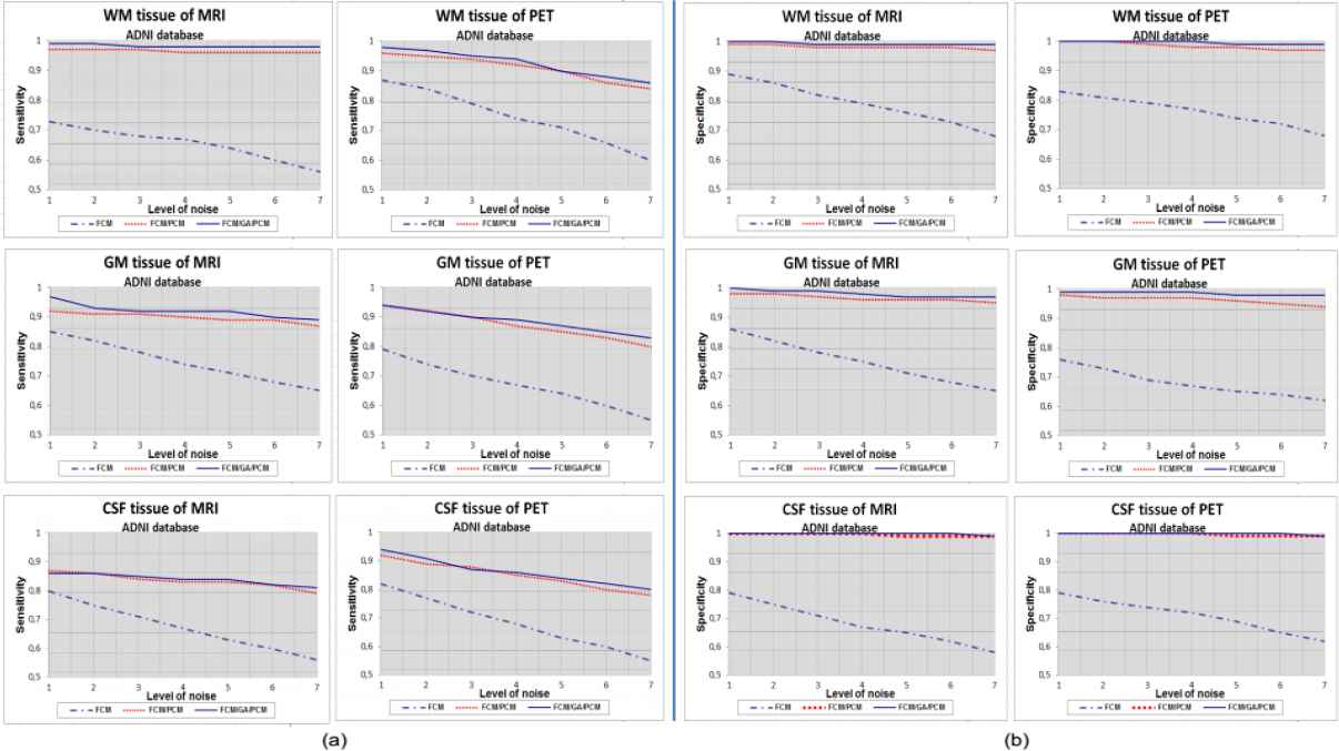
Curves of (a) sensitivity and (b) specificity clustering indexes for WM, GM and CSF tissue with 1%…7% SNR, using FCM, FCM/PCM and FCM/GA/PCM clustering algorithms, application for ADNI database.
Comparison of fuzzy tissue volumes of computed and reference labeled image with RF inhomogeneity = 20 %, slice thickness = 1 mm and SNR 7%, with using FCM/ GA /PCM, FCM/PCM and PCM clustering algorithms.
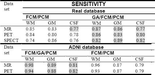
Sensitivity for WM, GM and CSF tissues with SNR = 7% using FCM/GA/PCM and FCM/PCM clustering algorithms.
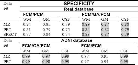
Specificity for WM, GM and CSF tissue with SNR = 7% using FCM/GA/PCM and FCM/PCM clustering algorithms.
It is evident from the tables (1, 2 and 3) and figures (4, 5 and 6) that for all images of the used techniques ensemble, the proposed hybrid FCM-AG-PCM clustering approach produces better scores compared to that produced by the other algorithms.
From Table 1., Tanimoto coefficients were excellent for all scan images, the TC obtained with the hybrid FCM/GA/PCM approach were better for all tissues than those resulting from FCM/PCM and conventional PCM algorithm.
From Table 2., the proposed hybrid algorithm provides the best results in terms of sensibility with SNR = 7, for all scan images.
Same diagnosis is in favor of the hybrid algorithm with respect to the results in Table 3. which represents the specificity.
From Fig. 4., Fig. 5. and Fig. 6., the quantitative evaluation with sensitivity and specificity validity measures prove the success of hybrid FCM/AG/PCM clustering scheme in quantifying volumes of brain tissue and performed well on most volumes from the real and synthetic data set. The result shown in figures demonstrates the robustness of this method in noisy environment (1% to 7%). We can also observed that for all tissues, the proposed hybrid FCM/AG/PCM clustering scheme produce better scores compared to that produced by the other algorithms used in the same conditions namely: FCM/PCM process and FCM clustering algorithm .
We can see from figures that FCM algorithm is not stable and very sensitive to noises in comparison with FCM/PCM or FCM/GA/PCM clustering approaches which gave generally stable values, but FCM/GA/PCM method gave more good performance and was stable.
Regarding the execution time, the GA/FCM/PCM algorithm consumed 7 s (for real images) and 6 s (for ADNI images) compared to 11 (for real images) and 9 s (for ADNI images) for the PCM algorithm.
So, the hybrid algorithm has converged more quickly compared to this fuzzy analog: conventional PCM algorithm. This is due to the empirical initialization of the centers of clusters with FCM/GA.
6. Conclusion and future work
The use of fuzzy logic for brain tissue segmentation is motivated by the fact that boundaries between brain tissues in the images are fuzzy rather than sharp [38]. Adding to this, noise, PVE or anatomical and functional variations within pure tissue activities introduce uncertainty and ambiguity [59].
We thus used a combination of fuzzy (FCM) and possibilistic (PCM) clustering algorithms to characterizing brain tissues from the anatomical and functional images, which the information in the images is carried out by the brain tissue distributions, revealing spatial locations in anatomical images (MRI) and distribution of a functional process in functional ones (SPECT, PET) [9]. The problem of fuzzy clustering has been posed as an optimization problem. So, we used GA to give cluster centers.
We model these tissue clusters by means of fuzzy maps, representing the distributions of possibility of tissues in the images. These maps assign a voxel to CSF, GM and WM with different absolute memberships, reflecting the way the voxel belongs to these tissues. To establish the superiority of the proposed hybrid clustering method, comparison has been made with several other well-known clustering algorithms.
As a part of the future, we think that the proposed hybrid clustering process based tissue modeling can be improved by fusion scheme which combines the advantage of anatomical image and those of functional image. We would be interesting to same fusion to reduce errors in tissue because, due to the noise and intensity inhomogeneity’s introduced in imaging process, different tissues at different locations may have similar intensity appearance, while the same tissue at different locations may have a different intensity appearance. We think that the fusion process could take in the count, the redundancy and ambiguity in images. We are currently working in this direction.
Footnotes
References
Cite this article
TY  - JOUR
AU  - Lilia Lazli
AU  - Mounir Boukadoum
PY  - 2018
DA  - 2018/04/30
TI  - Improvement of CSF, WM and GM Tissue Segmentation by Hybrid Fuzzy – Possibilistic Clustering Model based on Genetic Optimization Case Study on Brain Tissues of Patients with Alzheimer’s Disease
JO  - International Journal of Networked and Distributed Computing
SP  - 63
EP  - 77
VL  - 6
IS  - 2
SN  - 2211-7946
UR  - https://doi.org/10.2991/ijndc.2018.6.2.2
DO  - 10.2991/ijndc.2018.6.2.2
ID  - Lazli2018
ER  -