
Deep Learning–Based CT-to-CBCT Deformable Image Registration for Autosegmentation in Head and Neck Adaptive Radiation Therapy
 , Howard Morgan*, , Dan Nguyen, Steve Jiang
- DOI
- 10.2991/jaims.d.210527.001How to use a DOI?
- Keywords
- Deep learning; Deformable image registration; Segmentation; CBCT
- Abstract
The purpose of this study is to develop a deep learning–based method that can automatically generate segmentations on cone-beam computed tomography (CBCT) for head and neck online adaptive radiation therapy (ART), where expert-drawn contours in planning CT (pCT) images serve as prior knowledge. Because of the many artifacts and truncations that characterize CBCT, we propose to utilize a learning-based deformable image registration method and contour propagation to get updated contours on CBCT. Our method takes CBCT and pCT as inputs, and it outputs a deformation vector field and synthetic CT (sCT) simultaneously by jointly training a CycleGAN model and 5-cascaded Voxelmorph model. The CycleGAN generates the sCT from CBCT, while the 5-cascaded Voxelmorph warps the pCT to the sCT's anatomy. We compared the segmentation results to Elastix, Voxelmorph and 5-cascaded Voxelmorph models on 18 structures including target and organs-at-risk. Our proposed method achieved an average Dice similarity coefficient of 0.83 ± 0.09 and an average 95% Hausdorff distance of 2.01 ± 1.81 mm. Our method showed better accuracy than Voxelmorph and 5-cascaded Voxelmorph and comparable accuracy to Elastix, but with much higher efficiency. The proposed method can rapidly and simultaneously generate sCT with correct CT numbers and propagate contours from pCT to CBCT for online ART replanning.
- Copyright
- © 2021 The Authors. Published by Atlantis Press B.V.
- Open Access
- This is an open access article distributed under the CC BY-NC 4.0 license (http://creativecommons.org/licenses/by-nc/4.0/).
1. INTRODUCTION
Adaptive radiation therapy (ART) can improve the dosimetric quality of radiation therapy plans by altering the treatment plans based on patient anatomical changes [1]. However, the time-consuming parts of ART, including segmentation and re-planning, make online ART difficult to implement in clinics. Recently, several commercially available online ART systems have been developed: EthosTM (Varian Inc., Palo Alto, USA), MRIdianTM (ViewRay Inc., Cleveland, OH, USA) and UnityTM (Elekta AB Inc., Stockholm, Sweden). Ethos [2] is a cone-beam computed tomography (CBCT)-based online ART platform that works with Halcyon Linac, while MRIdian [3] and Unity [4] are magnetic resonance imaging (MRI)-based online ART platforms that work with MRI Linacs.
Even though MRI images have much better soft tissue contrast than CBCT images, CBCT images are often still used in ART because MRI's magnetic fields make it unsuitable for patients with metal implants, and MRI's expense make it unsuitable for clinics with value-based healthcare. As a tumor site that often has inter-fractional anatomical changes during RT, head and neck (H&N) cancer could benefit from CBCT-based online ART. A clinical study of ART benefits for H&N patients showed that it significantly reduced the dose to the parotid gland for all 30 patients [5]. Another study showed that target coverage for patients whose treatment plans were adapted improved by up to 10.7% of the median dose [6]. Thus, utilizing CBCT in an ART workflow can avoid the risk of underdose to the tumor and overdose to organs-at-risk (OARs).
To use CBCT in an ART workflow, corrections must be made to the CBCT. Compared to CT, CBCT has a lot of artifacts and inaccurate Hounsfield units (HU) values. To calculate the dose accurately on CBCT, HU values must be corrected, and artifacts must be removed from the CBCT. Our previous work used CycleGAN, a deep learning (DL)–based method, to convert CBCT to synthetic CT (sCT) images that have CT's HU values and fewer artifacts, and the dose distributions calculated on sCT showed a higher gamma index pass rate than those calculated on CBCT [7]. DL can generate sCT from CBCT for ART dose calculation more quickly, easily and accurately than deformable image registration (DIR) methods, because it doesn't require paired data for training, it enables rapid deployment of a trained mode, and it preserves the CBCT's anatomy.
Besides accurate dose calculation, another problem for using CBCT in online ART is achieving accurate autosegmentation. Because of the many artifacts and the axial truncation on CBCT images of H&N sites, using DL methods directly to contour OARs and the target on CBCT images is very challenging. One study used CycleGAN to convert CBCT to synthetic MRI images, then combined the CBCT and synthetic MRI together to enhance the training of a DL–based multi-organ autosegmentation model [8]. Most studies of autosegmenting from CBCT for online ART, as well as the state-of-the-art methods, still focus on DIR-based methods to get the deformation vector field (DVF) from warping the planning CT (pCT) to CBCT's anatomy, then applying the DVF to the contours on pCT to get the updated contours on CBCT [9]. However, DIR can generate inaccurate segmentations in cases with more pronounced anatomical changes or low soft tissue contrast [10].
Popular DIR methods include optical flow [11,12], b-spline based [13], demons [14], ANTs [15], and so on. Recently DL–based methods have gained lots of attention because their state-of-art performance in many applications. However, DL in medical image registration has not been extensively studied until four to five years ago [16]. A very important work that has been published by Jaderberg et al. in 2015 proposed a spatial transformer network (STN), which allows spatial transformations on the input image inside a neural network and is differentiable that can be added on any other existing architectures [17]. STN network has inspired lots of unsupervised DL–based DIR methods. A typical unsupervised DIR model can be divided into two parts: DVF prediction and spatial transformation. In DVF prediction, a neural network takes a pair of fixed and moving images as input and outputs a DVF. Then in spatial transformation, the STN network warps the moving images according to the predicted DVF to get the moved images. The loss function to train the model is usually composed of image similarity loss between the fixed and moved images and a regularization term on DVF. One of the popular unsupervised DL based DIR methods—Voxelmorph, combined a probabilistic generative model and a DL model for diffeomorphic registration [18]. Another similar work FAIM, used a U-Net architecture to predict DVF directly and a STN network to warp images [19]. VTN proposed by Zhao et al., integrated affine registration into the DIR network and added additional invertibility loss that encourages backward consistency [20].
It is reasonable to use contour propagation for autosegmentation in online ART, because DIR methods leverage prior knowledge from contours on pCT. DIR between daily/weekly CBCTs and pCTs is often used in H&N ART workflows to get the most up-to-date anatomy. Currently, the processes of CBCT-to-sCT conversion and pCT-to-CBCT DIR are always done separately. Therefore, we propose a method that combines a CycleGAN model and a DL–based DIR model together and jointly trains them. The CycleGAN model converts CBCT to sCT images, and the sCT generated is used by the DIR model for registration to the same imaging modality (sCT-to-CT), rather than across different imaging modalities (CBCT- to-CT). This is important, because DIR is considered more accurate within the same imaging modality than across different modalities [21]. The DIR model generates DVFs and deformed planning CTs (dpCT) by deforming the pCT to the sCT's anatomy, and the generated dpCT is used to guide CycleGAN to generate a more accurate sCT from CBCT during the CycleGAN training. A better quality sCT then leads to more accurate image registration. In this way, the two DL models can improve each other through their interaction, rather than training each alone. This method can also generate sCT from CBCT and updated contours from contour propagation at the same time for ART. Overall, we developed a method that can generate segmentations on CBCT and sCT from CBCT jointly, accurately, and efficiently.
2. DATA
We retrospectively collected data from 124 patients with H&N squamous cell carcinoma treated with external beam radiotherapy with a radiation dose around 70 Gy. Each patient case includes a pCT volume acquired before the treatment course, OAR and target segmentations delineated by physicians on the pCT and a CBCT volume acquired around fraction 20 during the treatment course. The pCT volumes were acquired by a Philips CT scanner with 1.17 × 1.17 × 3.00 mm3 voxel spacing. The CBCT volumes were acquired by Varian On-Board Imagers with 0.51 × 0.51 × 1.99 mm3 voxel spacing and 512 × 512 × 93 dimensions. The pCT was rigidly registered to the CBCT through Velocity (Varian Inc., Palo Alto, USA). Therefore, the rigid-registered pCT has the same voxel spacing and dimensions as the CBCT. After rigid registration, the dimensions of the pCT and CBCT volumes were both downsampled to 256 × 256 × 93 from 512 × 512 × 93, then cropped to 224 × 224 × 80. We divided the dataset into 100/4/20 for training/validation/testing, respectively. Since our proposed model is an unsupervised learning method, it does not need contours on pCT or ground truth contours on CBCT for training. However, we needed ground truth contours to evaluate the accuracy of the proposed DIR network. We selected 18 structures that are either critical OARs or have large anatomical changes during radiotherapy courses: left and right brachial plexus; brainstem; oral cavity; middle, superior, and inferior pharyngeal constrictor; esophagus; nodal gross tumor volume (nGTV); larynx; mandible; left and right masseter; left and right parotid gland; left and right submandibular gland; and spinal cord. The contours of the these 18 structures were first propagated from pCT to CBCT by using rigid and DIR in velocity, then they were modified and approved by a radiation oncologist to obtain the ground truth for validation and testing.
3. METHODS
3.1. Overview of CycleGAN
Our previous study used a CycleGAN architecture to convert CBCT to sCT images that have accurate HU values and fewer artifacts [7]. The architecture we used in the current study is shown in Figure 1. It has two generators with a U-Net architecture and two discriminators with a patchGAN architecture.

CycleGAN model architecture. The left figure is the architecture of CycleGAN and the right figure is the neural networks of the generators and discriminators used in the CycleGAN. Purple arrows illustrate the flow of one cycle and red arrows illustrate the flow of another cycle. Blue dashed lines connect the values used in the loss function.
The loss function for the discriminators is
For more details, the reader is referred to Liang et al. [7].
3.2. Overview of Voxelmorph
Recently, learning-based DIR methods have gained attention for their fast deployment compared to classical DIR techniques. One of the state-of-the-art networks is Voxelmorph [18]. This model assumes that the DVF can be defined by the following ordinary differential equation (ODE):


The architecture of Voxelmorph (a) and 5-cascaded Voxelmorph (b). The orange dashed lines illustrate the loss function.
3.3. 5-cascaded Voxelmorph
Recursive cascaded networks for DIR have been shown to significantly outperform state-of-the-art learning-based DIR methods [22]. Therefore, we used the 5-cascaded Voxelmorph network in this study to gain better DIR performance; its architecture is shown in Figure 2(b). The input of the 5-cascaded Voxelmorph is also pCT
The final warped images are constructed by
3.4. Joint Model
The performance of DIR highly depends on the image quality of the fixed and moving images. In our case, the image quality of the fixed images, which have a lot of artifacts and a different HU range from the moving images, is the main factor that causes DIR errors. Thus, we used sCT images generated by CycleGAN, which has fewer artifacts and a similar range of CT HU values, in place of CBCT as the fixed images. We propose a combined model that jointly trains CycleGAN and 5-cascaded Voxelmorph, as shown in Figure 3. With independently pretrained CycleGAN and 5-cascaded Voxelmorph models, we first update the parameters of the CycleGAN generators by using the loss function

The architecture of the joint model and its training scheme. Black dashed lines illustrate the loss function.
Unlike training CycleGAN alone, dpCT adds another supervision to guide CycleGAN to generate more realistic sCT images by adding
The more realistic the sCT images that CycleGAN generates, the more accurate the registration that DIR can perform. By jointly training CycleGAN and Voxelmorph, the two networks can improve each other for better results than training each separately.
3.5. Training Details
The CycleGAN, Voxelmorph, 5-cascaded Voxelmorph, and joint models were all trained with a volume size of 224 × 224 × 80 on an NVIDIA Tesla V100 GPU with 32 GB of memory. The maximum cascades we can have for the volume size of 224 × 224 × 80 and batch size of 1 without exceeding GPU memory capacity is 5. Adam optimization with a learning rate of 0.0002 was used for training all the models. Hyperparameters α, β,
3.6. Evaluation Methods
To quantitatively evaluate segmentation accuracy, we calculated the dice similarity coefficient (DSC), relative absolute volume difference (RAVD) and 95% Hausdorff distance (HD95). DSC gauges the similarity of the prediction and the ground truth by measuring the volumetric overlap between them. It is defined as
Like DSC, RAVD also measures volumetric discrepancies between the ground truth and the predicted segmentation. RAVD is defined as
HD is the maximum distance from a set to the nearest point in another set. It can be defined as
HD95 is based on the 95th percentile of the distances between boundary points in X and Y. The purpose of this metric is to avoid the impact of a small subset of the outliers.
We compared our proposed method, which is the joint model, with Voxelmorph and 5-cascaded Voxelmorph. We also compared the joint model with a non–learning-based state-of-the-art method. Elastix is a publicly available intensity-based medical image registration toolbox, extended from ITK [23].
4. RESULTS
The quantitative evaluation results—in terms of DSC, RAVD and HD95—between the predicted and the ground truth contours of the 18 structures for 20 test patients are shown in Table 1. Our proposed method achieved DSCs of 0.61, 0.63, 0.94, 0.94, 0.75, 0.72, 0.85, 0.80, 0.81, 0.89, 0.88, 0.91, 0.92, 0.91, 0.86, 0.79, 0.78 and 0.89 for left brachial plexus, right brachial plexus, brainstem, oral cavity, middle pharyngeal constrictor, superior pharyngeal constrictor, inferior pharyngeal constrictor, esophagus, nGTV, larynx, mandible, left masseter, right masseter, left parotid gland, right parotid gland, left submandibular gland, right submandibular gland and spinal cord, respectively. We calculated paired Student t tests for all metrics for statistical analysis (Table 2). Our proposed method outperformed Voxelmorph for all the structures except left brachial plexus and right brachial plexus. When compared to 5-cascaded Voxelmorph, our proposed method performed better on brainstem, oral cavity, middle pharyngeal constrictor, mandible, left masseter, right masseter, left parotid land, right parotid gland and right submandibular gland in at least one evaluation metric. Our proposed method performed comparably to Elastix on most of the 18 structures. However, its performance was superior to Elastix on mandible, esophagus and superior pharyngeal constrictor, and inferior to Elastix on left and right brachial plexus. For visual evaluation, Figures 4 and 5 shows segmentations of two test patients from Elastix, Voxelmorph, 5-cascaded Voxelmorph, the joint model and the ground truth, where similar phenomenon can be observed.
| Structure | Method | DSC | RAVD | HD95 (mm) |
|---|---|---|---|---|
| Left brachial plexus | Elastix | 0.80 ± 0.08 | 0.10 ± 0.07 | 1.27 ± 0.56 |
| Voxelmorph | 0.60 ± 0.18 | 0.14 ± 0.10 | 3.59 ± 2.01 | |
| 5-cascaded Voxelmorph | 0.65 ± 0.16 | 0.10 ± 0.08 | 3.10 ± 1.48 | |
| Joint model | 0.61 ± 0.18 | 0.12 ± 0.12 | 3.07 ± 2.74 | |
| Right brachial plexus | Elastix | 0.80 ± 0.08 | 0.10 ± 0.07 | 1.36 ± 0.70 |
| Voxelmorph | 0.60 ± 0.20 | 0.12 ± 0.09 | 3.76 ± 1.83 | |
| 5-cascaded Voxelmorph | 0.67 ± 0.16 | 0.09 ± 0.07 | 3.00 ± 1.42 | |
| Joint model | 0.63 ± 0.18 | 0.14 ± 0.11 | 2.92 ± 2.53 | |
| Brainstem | Elastix | 0.94 ± 0.03 | 0.01 ± 0.01 | 0.51 ± 0.00 |
| Voxelmorph | 0.89 ± 0.05 | 0.08 ± 0.06 | 1.94 ± 0.60 | |
| 5-cascaded Voxelmorph | 0.90 ± 0.04 | 0.03 ± 0.05 | 0.69 ± 0.58 | |
| Joint model | 0.94 ± 0.06 | 0.01 ± 0.02 | 0.66 ± 0.55 | |
| Oral cavity | Elastix | 0.95 ± 0.03 | 0.02 ± 0.02 | 1.62 ± 0.54 |
| Voxelmorph | 0.91 ± 0.04 | 0.05 ± 0.03 | 3.77 ± 1.31 | |
| 5-cascaded Voxelmorph | 0.92 ± 0.03 | 0.01 ± 0.03 | 1.74 ± 1.10 | |
| Joint model | 0.94 ± 0.04 | 0.01 ± 0.03 | 1.77 ± 1.15 | |
| Middle pharyngeal constrictor | Elastix | 0.73 ± 0.08 | 0.19 ± 0.10 | 2.62 ± 0.98 |
| Voxelmorph | 0.65 ± 0.15 | 0.16 ± 0.13 | 4.22 ± 2.53 | |
| 5-cascaded Voxelmorph | 0.71 ± 0.10 | 0.11 ± 0.10 | 2.07 ± 2.21 | |
| Joint model | 0.75 ± 0.12 | 0.10 ± 0.12 | 2.00 ± 2.25 | |
| Superior pharyngeal constrictor | Elastix | 0.68 ± 0.12 | 0.27 ± 0.13 | 2.66 ± 1.31 |
| Voxelmorph | 0.66 ± 0.10 | 0.15 ± 0.11 | 3.50 ± 2.69 | |
| 5-cascaded Voxelmorph | 0.72 ± 0.08 | 0.13 ± 0.09 | 1.62 ± 1.63 | |
| Joint model | 0.72 ± 0.08 | 0.12 ± 0.12 | 1.78 ± 2.13 | |
| Inferior pharyngeal constrictor | Elastix | 0.83 ± 0.06 | 0.13 ± 0.10 | 2.23 ± 0.52 |
| Voxelmorph | 0.72 ± 0.13 | 0.17 ± 0.14 | 3.98 ± 1.94 | |
| 5-cascaded Voxelmorph | 0.83 ± 0.10 | 0.13 ± 0.14 | 2.10 ± 1.33 | |
| Joint model | 0.85 ± 0.12 | 0.12 ± 0.13 | 2.11 ± 1.86 | |
| Esophagus | Elastix | 0.85 ± 0.08 | 0.09 ± 0.08 | 1.77 ± 0.36 |
| Voxelmorph | 0.75 ± 0.15 | 0.19 ± 0.16 | 3.33 ± 2.11 | |
| 5-cascaded Voxelmorph | 0.80 ± 0.10 | 0.11 ± 0.08 | 1.69 ± 0.95 | |
| Joint model | 0.80 ± 0.10 | 0.09 ± 0.08 | 1.67 ± 1.67 | |
| nGTV | Elastix | 0.81 ± 0.07 | 0.13 ± 0.13 | 2.53 ± 1.07 |
| Voxelmorph | 0.67 ± 0.12 | 0.36 ± 0.21 | 6.19 ± 3.38 | |
| 5-cascaded Voxelmorph | 0.82 ± 0.11 | 0.12 ± 0.22 | 2.83 ± 3.52 | |
| Joint model | 0.81 ± 0.11 | 0.13 ± 0.22 | 2.89 ± 3.51 | |
| Larynx | Elastix | 0.89 ± 0.06 | 0.07 ± 0.10 | 3.60 ± 2.75 |
| Voxelmorph | 0.82 ± 0.11 | 0.07 ± 0.05 | 5.53 ± 3.30 | |
| 5-cascaded Voxelmorph | 0.88 ± 0.08 | 0.06 ± 0.06 | 3.70 ± 2.99 | |
| Joint model | 0.89 ± 0.09 | 0.07 ± 0.06 | 3.66 ± 3.22 | |
| Mandible | Elastix | 0.87 ± 0.05 | 0.15 ± 0.10 | 2.19 ± 0.82 |
| Voxelmorph | 0.85 ± 0.06 | 0.21 ± 0.12 | 2.48 ± 1.05 | |
| 5-cascaded Voxelmorph | 0.87 ± 0.04 | 0.18 ± 0.11 | 1.97 ± 0.92 | |
| Joint model | 0.88 ± 0.05 | 0.14 ± 0.10 | 1.88 ± 0.97 | |
| Left masseter | Elastix | 0.90 ± 0.04 | 0.05 ± 0.03 | 1.49 ± 0.39 |
| Voxelmorph | 0.86 ± 0.04 | 0.06 ± 0.05 | 2.39 ± 0.69 | |
| 5-cascaded Voxelmorph | 0.87 ± 0.03 | 0.06 ± 0.05 | 1.46 ± 0.66 | |
| Joint model | 0.91 ± 0.03 | 0.04 ± 0.06 | 1.36 ± 0.52 | |
| Right masseter | Elastix | 0.91 ± 0.03 | 0.04 ± 0.04 | 1.53 ± 0.41 |
| Voxelmorph | 0.87 ± 0.04 | 0.11 ± 0.09 | 2.36 ± 0.75 | |
| 5-cascaded Voxelmorph | 0.89 ± 0.03 | 0.09 ± 0.07 | 1.19 ± 0.34 | |
| Joint model | 0.92 ± 0.02 | 0.08 ± 0.07 | 1.20 ± 0.50 | |
| Left parotid gland | Elastix | 0.89 ± 0.07 | 0.06 ± 0.07 | 1.67 ± 0.92 |
| Voxelmorph | 0.81 ± 0.07 | 0.18 ± 0.18 | 4.18 ± 2.37 | |
| 5-cascaded Voxelmorph | 0.88 ± 0.07 | 0.08 ± 0.11 | 1.03 ± 2.37 | |
| Joint model | 0.91 ± 0.07 | 0.07 ± 0.10 | 1.06 ± 2.36 | |
| Right parotid gland | Elastix | 0.88 ± 0.08 | 0.07 ± 0.08 | 1.93 ± 0.99 |
| Voxelmorph | 0.77 ± 0.09 | 0.26 ± 0.21 | 5.01 ± 2.21 | |
| 5-cascaded Voxelmorph | 0.86 ± 0.09 | 0.08 ± 0.05 | 1.92 ± 2.26 | |
| Joint model | 0.86 ± 0.09 | 0.07 ± 0.05 | 1.76 ± 2.20 | |
| Left submandibular gland | Elastix | 0.81 ± 0.11 | 0.10 ± 0.09 | 2.13 ± 0.76 |
| Voxelmorph | 0.74 ± 0.12 | 0.20 ± 0.14 | 3.77 ± 1.57 | |
| 5-cascaded Voxelmorph | 0.79 ± 0.12 | 0.15 ± 0.11 | 2.63 ± 1.74 | |
| Joint model | 0.79 ± 0.13 | 0.15 ± 0.13 | 2.66 ± 1.78 | |
| Right submandibular gland | Elastix | 0.83 ± 0.09 | 0.11 ± 0.13 | 2.25 ± 1.10 |
| Voxelmorph | 0.70 ± 0.13 | 0.20 ± 0.19 | 4.15 ± 1.99 | |
| 5-cascaded Voxelmorph | 0.78 ± 0.12 | 0.14 ± 0.11 | 2.97 ± 1.98 | |
| Joint model | 0.78 ± 0.13 | 0.14 ± 0.22 | 2.82 ± 1.93 | |
| Spinal cord | Elastix | 0.91 ± 0.04 | 0.01 ± 0.02 | 0.74 ± 0.99 |
| Voxelmorph | 0.85 ± 0.04 | 0.10 ± 0.10 | 2.58 ± 1.08 | |
| 5-cascaded Voxelmorph | 0.89 ± 0.04 | 0.04 ± 0.05 | 0.92 ± 0.86 | |
| Joint model | 0.89 ± 0.04 | 0.03 ± 0.05 | 0.95 ± 0.70 | |
| Elastix | 0.85 ± 0.07 | 0.09 ± 0.08 | 1.89 ± 0.84 | |
| Voxelmorph | 0.76 ± 0.10 | 0.16 ± 0.12 | 3.71 ± 1.86 | |
| Average | 5-cascaded Voxelmorph | 0.82 ± 0.08 | 0.10 ± 0.09 | 2.04 ± 1.57 |
| Joint model | 0.83 ± 0.09 | 0.09 ± 0.10 | 2.01 ± 1.81 |
Quantitative evaluation of segmentations by Elastix, Voxelmorph, 5-cascaded Voxelmorph and the joint model with DSC, RAVD and HD95 metrics. The values in the table are mean ± SD.
| Structure | Method | DSC | RAVD | HD95 |
|---|---|---|---|---|
| Left brachial plexus | Elastix vs. joint model | <0.01 | 0.46 | <0.01 |
| Voxelmorph vs. joint model | 0.36 | 0.52 | 0.30 | |
| 5-cascaded Voxelmorph vs. joint model | <0.01 | 0.28 | 0.96 | |
| Right brachial plexus | Elastix vs. joint model | <0.01 | 0.20 | 0.02 |
| Voxelmorph vs. joint model | 0.07 | 0.59 | 0.11 | |
| 5-cascaded Voxelmorph vs. joint model | <0.01 | 0.09 | 0.88 | |
| Brainstem | Elastix vs. joint model | 0.73 | 0.46 | 0.26 |
| Voxelmorph vs. joint model | <0.01 | <0.01 | <0.01 | |
| 5-cascaded Voxelmorph vs. joint model | <0.01 | 0.04 | 0.81 | |
| Oral cavity | Elastix vs. joint model | 0.57 | 0.48 | 0.49 |
| Voxelmorph vs. joint model | <0.01 | <0.01 | <0.01 | |
| 5-cascaded Voxelmorph vs. joint model | <0.01 | 0.66 | 0.43 | |
| Middle pharyngeal constrictor | Elastix vs. joint model | 0.31 | 0.05 | 0.20 |
| Voxelmorph vs. joint model | <0.01 | 0.04 | <0.01 | |
| 5-cascaded Voxelmorph vs. joint model | 0.03 | 0.58 | 0.93 | |
| Superior pharyngeal constrictor | Elastix vs. joint model | 0.13 | <0.01 | 0.14 |
| Voxelmorph vs. joint model | <0.01 | 0.09 | <0.01 | |
| 5-cascaded Voxelmorph vs. joint model | 0.80 | 0.72 | 0.37 | |
| Inferior pharyngeal constrictor | Elastix vs. joint model | 0.64 | 0.97 | 0.74 |
| Voxelmorph vs. joint model | <0.01 | 0.06 | <0.01 | |
| 5-cascaded Voxelmorph vs. joint model | 0.12 | 0.91 | 0.97 | |
| Esophagus | Elastix vs. joint model | 0.02 | 0.25 | 0.80 |
| Voxelmorph vs. joint model | 0.03 | 0.06 | <0.01 | |
| 5-cascaded Voxelmorph vs. joint model | 0.59 | 0.65 | 0.95 | |
| nGTV | Elastix vs. joint model | 0.96 | 0.96 | 0.73 |
| Voxelmorph vs. joint model | <0.01 | <0.01 | <0.01 | |
| 5-cascaded Voxelmorph vs. joint model | 0.46 | 0.12 | 0.29 | |
| Larynx | Elastix vs. joint model | 0.88 | 0.71 | 0.89 |
| Voxelmorph vs. joint model | <0.01 | 0.47 | <0.01 | |
| 5-cascaded Voxelmorph vs. joint model | 0.55 | 0.60 | 0.84 | |
| Mandible | Elastix vs. joint model | 0.05 | 0.43 | 0.02 |
| Voxelmorph vs. joint model | <0.01 | <0.01 | <0.01 | |
| 5-cascaded Voxelmorph vs. joint model | 0.45 | <0.01 | 0.05 | |
| Left masseter | Elastix vs. joint model | 0.30 | 0.70 | 0.44 |
| Voxelmorph vs. joint model | <0.01 | 0.03 | <0.01 | |
| 5-cascaded Voxelmorph vs. joint model | <0.01 | 0.01 | 0.23 | |
| Right masseter | Elastix vs. joint model | 0.18 | 0.23 | 0.08 |
| Voxelmorph vs. joint model | <0.01 | 0.01 | <0.01 | |
| 5-cascaded Voxelmorph vs. joint model | <0.01 | <0.01 | 0.93 | |
| Left parotid gland | Elastix vs. joint model | 0.14 | 0.88 | 0.23 |
| Voxelmorph vs. joint model | <0.01 | <0.01 | <0.01 | |
| 5-cascaded Voxelmorph vs. joint model | <0.01 | 0.36 | 0.41 | |
| Right parotid gland | Elastix vs. joint model | 0.21 | 0.76 | 0.99 |
| Voxelmorph vs. joint model | <0.01 | <0.01 | <0.01 | |
| 5-cascaded Voxelmorph vs. joint model | <0.01 | 0.74 | <0.01 | |
| Left submandibular gland | Elastix vs. joint model | 0.08 | 0.18 | 0.26 |
| Voxelmorph vs. joint model | <0.01 | 0.23 | <0.01 | |
| 5-cascaded Voxelmorph vs. joint model | 0.70 | 0.97 | 0.44 | |
| Right submandibular gland | Elastix vs. joint model | 0.13 | 0.46 | 0.15 |
| Voxelmorph vs. joint model | <0.01 | 0.04 | <0.01 | |
| 5-cascaded Voxelmorph vs. joint model | 0.97 | 0.92 | <0.01 | |
| Spinal cord | Elastix vs. joint model | 0.06 | 0.46 | 0.62 |
| Voxelmorph vs. joint model | <0.01 | 0.08 | <0.01 | |
| 5-cascaded Voxelmorph vs. joint model | 0.74 | 0.91 | 0.95 |
P-values of paired Student t-tests for Elastix versus joint model, Voxelmorph versus joint model and 5-cascaded Voxelmorph versus joint model.


The autosegmentation results on CBCT. The background images are CBCT. The rows from top to bottom are segmentation results by different methods. Those methods are (a) Elastix, (b) Voxelmorph, (c) 5-cascaded Voxelmorph, (d) joint model and (e) ground truth for a test patient on axial view. Different colors represent different structures which are illustrated in the legend.

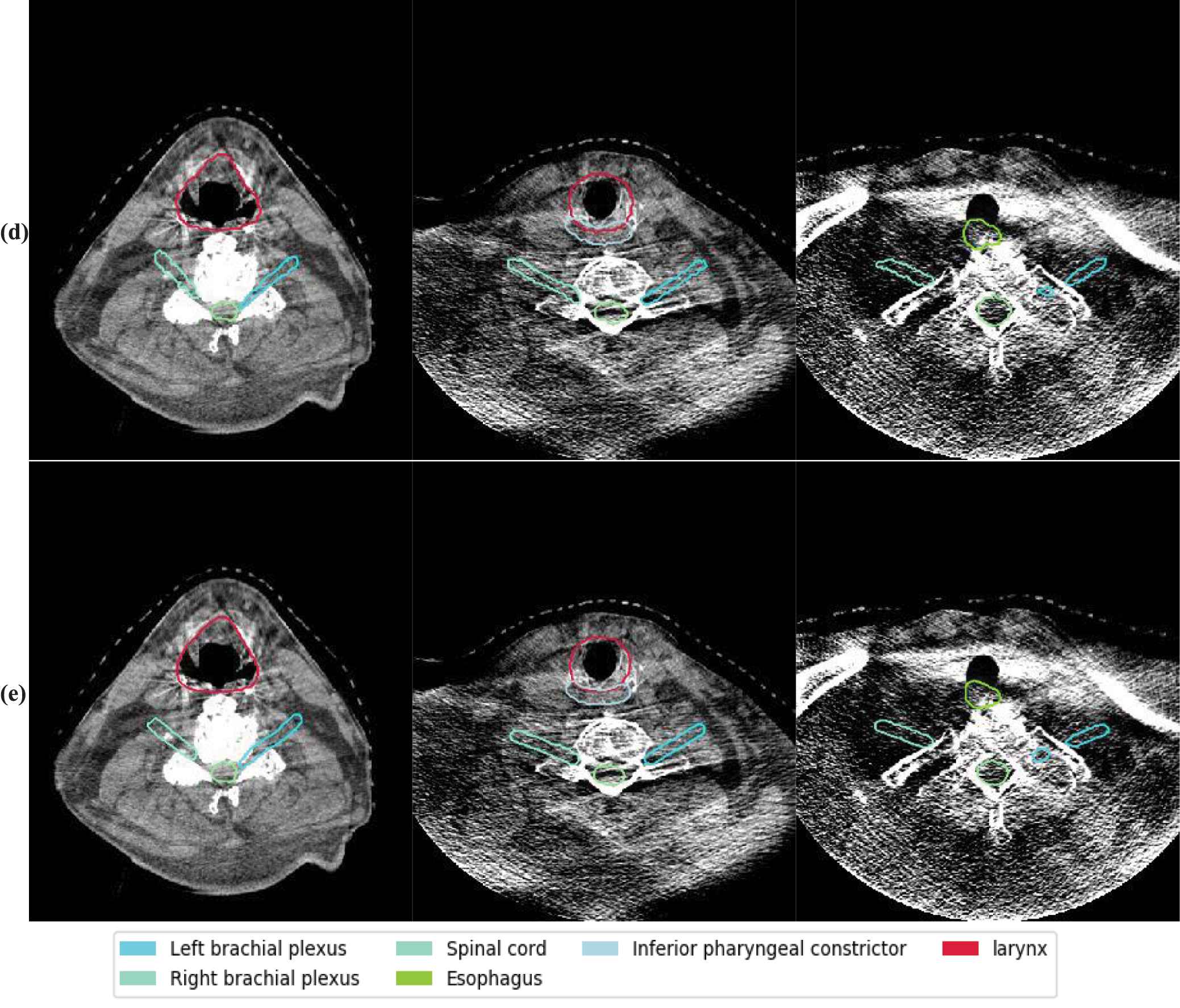
The autosegmentation results on CBCT. The background images are CBCT. The rows from top to bottom are segmentation results by different methods. Those methods are (a) Elastix, (b) Voxelmorph, (c) 5-cascaded Voxelmorph, (d) joint model and (e) ground truth for a test patient on axial view. Different colors represent different structures which are illustrated in the legend.
5. DISCUSSION AND CONCLUSION
The sCT images generated by the CycleGAN model trained alone and the CycleGAN model trained jointly with 5-cascaded Voxelmorph are shown in Figure 6. This shows that sCT images generated by the joint model are smoother than sCT images generated by CycleGAN alone. This phenomenon accords with the assumption that adding dpCT in the CycleGAN loss function would introduce patient-specific knowledge to guide training, while the CycleGAN trained alone lacks this information because of the unpaired training scheme. Consequently, better sCT image quality can be achieved by jointly training, and doing so results in more accurate image registration. Therefore, the joint model can outperform 5-cascaded Voxelmorph on some structures.
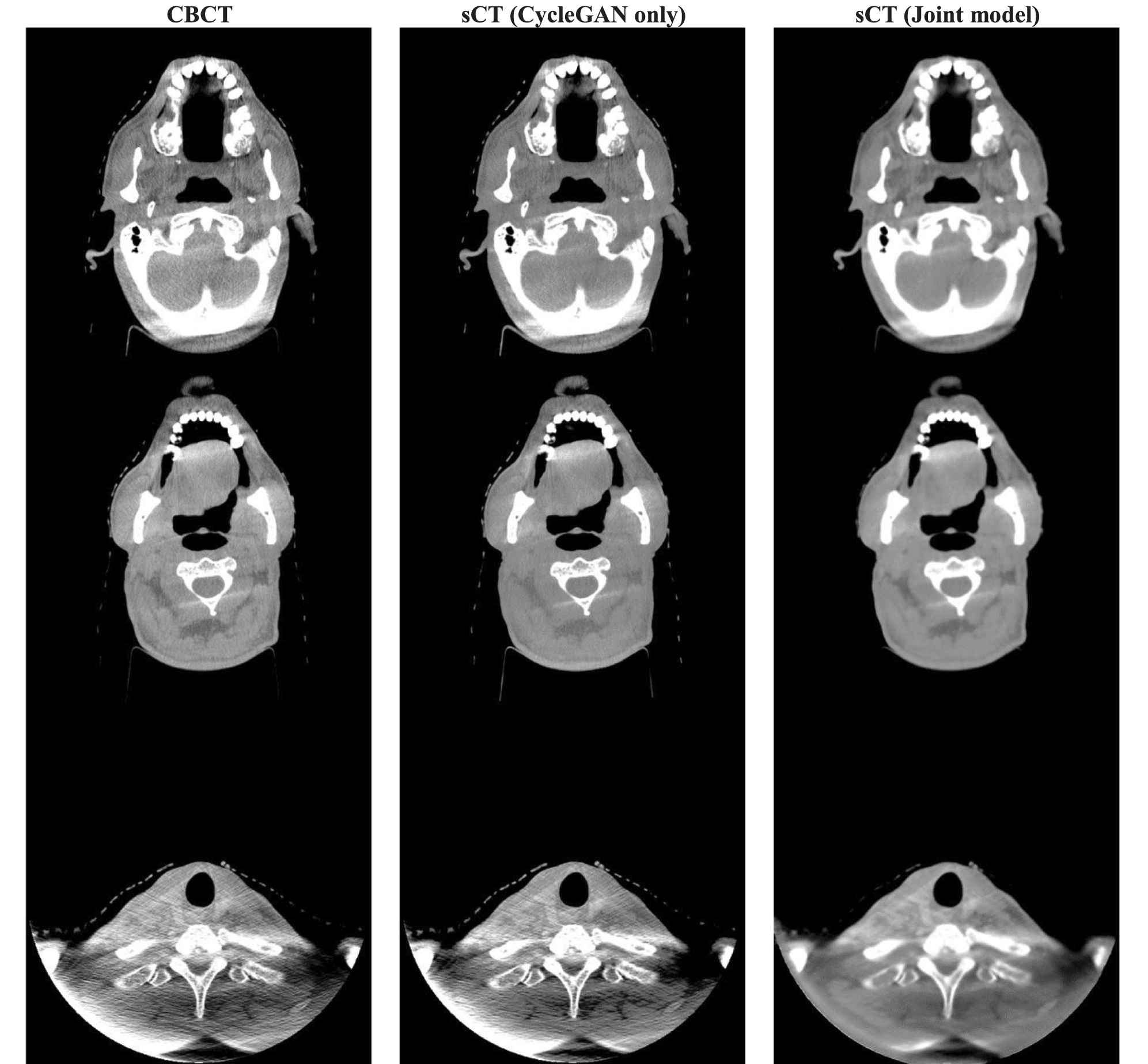
Axial view of CBCT and sCT images. From left to right, the images are CBCT, sCT generated by CycleGAN only and sCT generated by the joint model. HU window is (−500, 500).
However, we did not see the learning-based methods surpass the traditional DIR method. For most of the structures, our proposed method was comparable to Elastix. Despite better performance on mandible, esophagus and superior pharyngeal constrictor, the joint model nevertheless performed worse on left and right brachial plexus. This was because of an oversmooth sCT and because the structure itself was vague on CT images. However, the joint model after training can be completed in a minute for each patient, which is much faster than Elastix. In online ART workflows, where time is limited, the DL–based method is, thus, more suitable than Elastix.
One limitation of our method is its generalizability. According to our previous study, a CycleGAN trained on CBCTs from one distribution may not work on CBCTs from another distribution [24]. Thus, the proposed model needs to be retrained or fine-tuned before being deployed in other institutions. Another issue needs to pay attention to is how to stabilize neural networks especially GAN-based neural networks are well known for their instability. Some research have been focused on this issue. One of the classical papers used their proposed analytic compressive iterative deep framework to stabilize deep image reconstruction such that the neural networks would keep stabilized against input perturbation, adversarial attacks and more input data [25].
In conclusion, we developed a learning-based DIR method for contour propagation that can be used in ART. The proposed method can generate sCTs with correct CT numbers for dose calculation and, at the same time, rapidly propagate the contours from pCT to CBCT for treatment replanning. As such, this is a promising tool for external beam online ART.
DATA AVAILABILITY
All datasets were collected from one institution and are nonpublic. According to HIPAA policy, access to the dataset will be granted on a case by case basis upon submission of a request to the corresponding authors and the institution.
CONFLICT OF INTERESTS
The authors declare no competing financial interest. The authors confirm that all funding sources supporting the work and all institutions or people who contributed to the work, but who do not meet the criteria for authorship, are acknowledged. The authors also confirm that all commercial affiliations, stock ownership, equity interests or patent licensing arrangements that could be considered to pose a financial conflict of interest in connection with the work have been disclosed.
AUTHORS' CONTRIBUTIONS
Steve Jiang: Initiated the project; Xiao Liang, Howard Morgan, Dan Nguyen and Steve Jiang: Designed the experiments; Xiao Liang: Performed the model training, data analysis, and wrote the paper; Howard Morgan: Conducted the data collection and manual segmentation, Steve Jiang: Edited the paper.
Funding Statement
This work was supported by Varian Medical Systems, Inc.
ACKNOWLEDGMENTS
We would like to thank Varian Medical Systems, Inc., for supporting this study and Dr. Jonathan Feinberg for editing the manuscript.
REFERENCES
Cite this article
TY  - JOUR
AU  - Xiao Liang
AU  - Howard Morgan
AU  - Dan Nguyen
AU  - Steve Jiang
PY  - 2021
DA  - 2021/06/10
TI  - Deep Learning–Based CT-to-CBCT Deformable Image Registration for Autosegmentation in Head and Neck Adaptive Radiation Therapy
JO  - Journal of Artificial Intelligence for Medical Sciences
SP  - 62
EP  - 75
VL  - 2
IS  - 1-2
SN  - 2666-1470
UR  - https://doi.org/10.2991/jaims.d.210527.001
DO  - 10.2991/jaims.d.210527.001
ID  - Liang2021
ER  -