
Is it Export- or Import-Led Growth? The Case of Kenya
The paper was written while on secondment by UNU-WIDER to Uongozi Institute, Tanzania. The author’s institutional affiliation changed to Research Department, Central Bank of Kenya.
- DOI
- 10.2991/jat.k.210818.001How to use a DOI?
- Keywords
- Trade; export-led growth; import; import substitution; Kenya
- Abstract
The role of exports in promoting economic growth has been widely acknowledged. This paper analyses the link between exports, imports, and growth performance in Kenya using time series data. Despite trade liberalization and export promotion policies pursued over time, Kenya’s export growth has been sluggish, and exports are still strongly geared towards primary agricultural goods. Furthermore, empirical results show that aggregate exports have no statistically significant effect on output growth; instead, output growth is influenced by imports. Moreover, the diversification of imports has a larger impact on output growth than export diversification. Although analysis using disaggregated data shows a positive impact of machinery exports on output growth, the impact is smaller than that of imported manufactured and agricultural commodities. Therefore, the results generally suggest import-led growth and not export-led growth, signifying the economy’s dependence on imports. There is a need for Kenya to revamp the export-led growth strategy by enhancing export competitiveness, increasing value-addition, export diversification, and leveraging on regional and global value chains.
- Copyright
- © 2021 African Export-Import Bank. Publishing services by Atlantis Press International B.V.
- Open Access
- This is an open access article distributed under the CC BY-NC 4.0 license (http://creativecommons.org/licenses/by-nc/4.0/).
1. INTRODUCTION
The role of exports in promoting economic growth has been brought to the fore by the new wave of openness to trade as an economic strategy for development. Ideally, increased openness enables domestic producers to access the larger market for domestic goods, facilitating economies of scale in producing goods and services (Pistoresi and Rinaldi, 2012). Promoting exports encourages specialization and learning-by-doing, increasing productivity in the tradable sector and the entire economy (Krugman, 1995; Kinuthia, 2016). The improvement in productivity increases the competitiveness and profitability of enterprises. This provides incentives for domestic producers to increase production. In this regard, increasing exports fosters economic growth.
However, Export-Led Growth (ELG) is elusive and seemingly a mirage for many low-income and developing African countries. Firstly, the reliance on free trade and exports as a catalyst of economic growth in developing countries has been impeded by the export of primary goods, which tend to be associated with little innovation and low productivity. As a result, factor earnings in the primary sector are low, and the sector militates against overall productivity improvement, with weak backward and forward linkages (Krugman, 1995; Fosu, 1996; Krueger, 1997).1 Secondly, due to relatively low prices and high competition, primary exports tend to be associated with deteriorating terms of trade and a worsening balance of payments between developed and developing countries. Thirdly, primary goods have low-income elasticity. Consequently, the quantity of exports does not increase with the growth in trading partners’ incomes. Fourthly, despite the notable reduction of tariff and non-tariff barriers, nationalistic sentiments and rising agitation for greater protectionism have curtailed the growth of exports to developing and developed economies. Examples include the exit of the United Kingdom from the European Union, the protectionist trade policy by the USA and emerging economies, and the slow pace of economic integration and intricacies in the East African Community (EAC). Thus, many developing African economies have not realized expected economic growth by increasing the volume of exports (Santos-Paulino and Thirlwall, 2004; Were, 2015). Industrialization policy has also not used export promotion strategies to develop the industrial sector to increase the share of manufactured goods in exports and national output (Krueger, 1997; UNCTAD, 2017). Challenges to ELG are further compounded by domestic trade policies and supply-side constraints (UNECA, 2017).
Despite ELG challenges, Kenya shifted its trade strategy from Import Substitution (IS) to export promotion and trade openness since 1990 by significantly reducing restrictions to international trade (Adam et al., 2010; Were et al., 2006). Furthermore, Kenya is actively engaged in regional and continental integration initiatives aimed at enhancing trade. However, notwithstanding increased integration, extensive liberalization, and adoption of an outward-oriented policy, Kenya’s exports have neither increased substantially nor has a robust ELG been realized akin to Asian countries pursuing ELG policies (UNCTAD, 2017). Instead, imports have not only grown in tandem with economic growth, but they have also exceeded the export growth rate. The rapid growth of imports amid weak export performance has reignited the debate on the relative roles of exporting and importing as a catalyst of structural transformation to hasten economic growth (Kinuthia, 2016; Mazumdar, 2001). Although there is ample empirical evidence for ELG, there is scant evidence regarding the export–growth nexus for African countries like Kenya.
It is against this background that this paper analyses the relationship between exports, imports, and growth in Kenya. Kenya is a good case because, firstly, inward- and outward-oriented policies have been implemented for a significant period of time. Secondly, efforts to enhance trade volume and output through trade integration initiatives such as the EAC, Common Market for Eastern and Southern Africa (COMESA), and African Continental Free Trade Area (AfCFTA) make the assessment of the relationship between exports and growth even more pertinent. Thirdly, Kenya’s long-term development vision of becoming an industrialized economy by 2030 is underpinned by an outward trade-oriented growth strategy. The export sector, in particular, is expected to contribute significantly to the economic transformation needed to achieve a targeted economic growth rate of 10% annually.
We use cointegration analysis to establish the relative effect of exports and imports on growth using time series data from 1960 to 2019. The analysis shows that exports mainly consist of primary agricultural goods, and their contribution to growth is small. The empirical analysis indicates that the impact of aggregate exports on economic growth is not statistically significant. Imports largely influence aggregate and sectoral output growth, notwithstanding the short-run negative impact of imported agricultural commodities and imported machinery that denote a crowding-out effect of domestic production. Similarly, the diversity of imports has a larger effect on growth than the diversity of exports. Besides imports, total factor productivity and capital formation also promote growth. Moreover, imports and manufactured output have a positive impact on exports. However, analysis using disaggregated exports and imports data shows that machinery exports positively impact growth. In general, empirical evidence is more aligned to Import-Led Growth (ILG). Imports affect output and export growth as they generate productivity spillovers in the economy, emanating from imported intermediate and capital goods. These findings are consistent with Romer (1986, 1989) and Mazumdar (2001). Nonetheless, there is a need to rethink the envisioned ELG strategy.
The rest of the paper is organized as follows. An overview of Kenya’s trade policies and export performance is presented in Section 2. Section 3 reviews the literature on the relationship between exports and economic growth, while Section 4 outlines the theoretical framework. Section 5 describes the empirical model and data used. The exploratory analysis and empirical results are reported in Section 6, while Section 7 provides the conclusion and policy implications.
2. AN OVERVIEW OF KENYA’S TRADE POLICIES AND EXPORT PERFORMANCE
Kenya’s trade policy transitioned from an IS strategy at independence in 1963 to an export-promotion strategy in the early 1990s. Domestic industries and IS protectionism were first entrenched in the economy by the Foreign Investment Act of 1964. Key elements of this Act were the sanctity of private property and the protection of multinational corporations operating in Kenya from foreign competition. Thus, the Act anchored IS strategy as a trade policy in Kenyan laws. In addition to the Foreign Investment Act, sessional paper number 10 of 1965 on African Socialism and its Application for Planning in Kenya affirmed protection of private investment from state expropriation and domestic investment from foreign competition. More importantly, the policy paper stipulated that the limited foreign reserves available were to be utilized to buy capital goods to produce hitherto imported goods and, if possible, export some of the output (Were et al., 2006; Adam et al., 2010).
As a result of IS, manufacturing output growth averaged about 10% between 1964 and 1970, while exports and the Gross Domestic Product (GDP) growth rates were between 5% and 8%, implying that the manufacturing sector was contributing significantly to economic growth. This encouraged the government to increase tariff and non-tariff barriers to protect industries, coupled with investment incentives to enhance IS (KNBS, 1971; Reinikka, 1996).
However, despite the incentives, enterprises failed to grow to realize their full potential. The IS strategy was counterproductive in the industrial sector and the agricultural sector, as inputs became expensive. Domestic firms were less exposed to foreign competition; therefore, they neither had an incentive to innovate to produce competitively nor benefitted from foreign technological advancement. This contributed to the decline in the competitiveness of exports. The loss of competitiveness was more pronounced in the manufacturing sector compared to the agricultural sector. The decline in global commodity prices after the oil crises of 1973 and 1979 exposed more weaknesses of the control regime. Imports of intermediate goods declined, manufacturing firms operated at less than 40% of capacity. In addition, the manufacturing sector’s share of value-added output in GDP reduced from 10% to 8% between 1970 and 1992 (Reinikka, 1996). The dismal performance of the manufacturing and agricultural sectors partly contributed to a slower GDP growth rate of 0.4% in 1992, given their significant contribution to overall output (Figure 1).
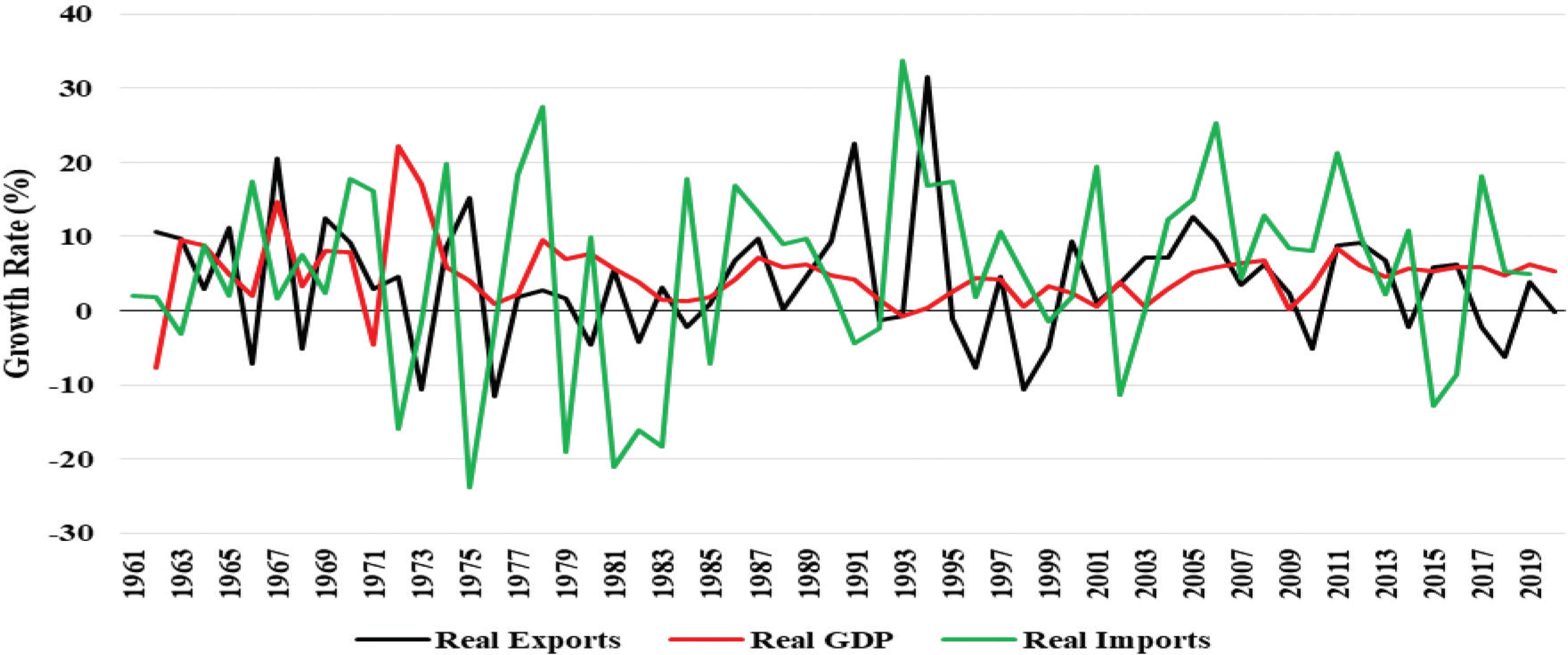
Export performance and economic growth. Source: Authors’ illustration based on data from World Development Indicators (World Bank, 2019).
Economic liberalization reforms were instituted to resuscitate the economy in response to receding growth. The main economic reforms toward trade liberalization included price decontrols, removal of tariff and non-tariff barriers, and adoption of export promotion initiatives (Were et al., 2006). Initiatives instituted to promote exports included manufacturing under bond and export processing zones, investment incentives and increasing exports markets through regional integration and signing bilateral trade agreements (Adam et al., 2010).
Although the manufacturing sector’s output growth rate increased from 1.2% in 1992 to over 3.9% in 1996, as the overall GDP growth rate increased to 4.6%, the growth of exports decelerated (KNBS, 2019). Over the period from 1993 to 2000, the export sector performed poorly even for commodity exports such as tea, coffee, and horticulture, in which Kenya has a comparative advantage (Figure 2). This may have been partly due to structural bottlenecks and non-tariff barriers that still constrained international trade despite extensive liberalization of the economy. Moreover, inconsistent implementation of trade policy over this period increased the economy’s risk profile, thus discouraging domestic and foreign direct investment (Reinikka, 1996; Adam et al., 2010).
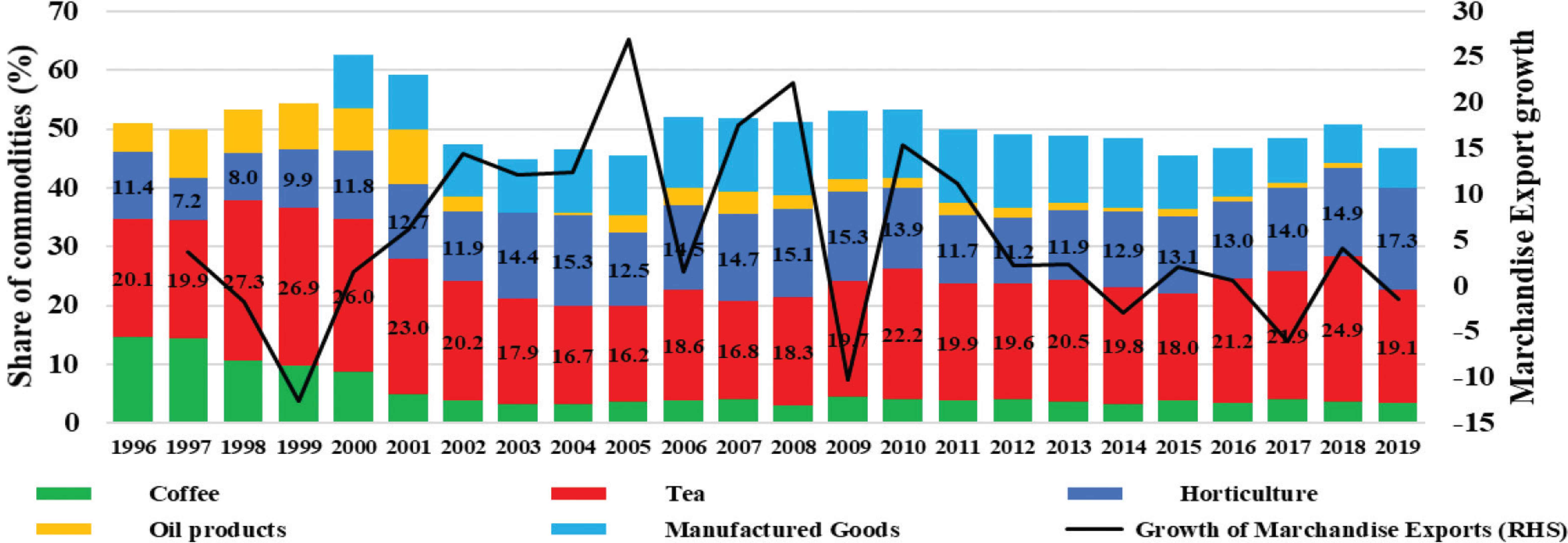
Total merchandise exports and major export commodities growth rate. Source: Authors’ illustration based on Central Bank of Kenya (CBK) data (CBK, 2020).
Following the economic downturn of between 1995 and 2001, the Economic Recovery Strategy Paper for Wealth and Employment Creation for 2003–2007 was launched as a medium-term plan to restructure and revamp the economy. Trade and industry, especially small- and medium-sized enterprises and the export sector, were to be resuscitated to increase the share of manufactured goods and services, and the diversity of exports. As a result, the nominal exports growth rate increased from an average of 4.1% between 1990 and 1999 to 11% between 2000 and 2009.
Despite export promotion strategies, such as horticulture and apparel exports under Economic Partnership Agreement and the African Growth and Opportunity Act,2 respectively, the performance of Kenya’s exports has been dismal. The value of the export growth rate averaged 11%, while the number of exports grew by 1.6% between 2000 and 2010. However, primary commodities dominated exports, and the value of imports increased at an average rate of 8.8%, corresponding to a quantity growth rate of 2.8% over the same period. The poor performance of export growth vis-à-vis import growth widened the trade gap to an average growth rate of 8.3% between 2000 and 2010 period, and the gap is still wide (Figure 3).

Trade gap. Source: Authors’ illustration based on World Bank data (World Bank, 2019).
Notwithstanding efforts toward export diversification beyond agricultural products such as tea, coffee, and horticulture, the range of manufactured exports is narrow. As a result, agricultural exports still dominate Kenya’s merchandise exports. For instance, in 2016, the share of manufactured exports was 17.5% compared to 42.9% for agriculture exports (Figure 4). Agricultural exports include tea, coffee, and animal products, which have low prices and income elasticity. As a result, they yield lower and volatile foreign earnings compared to manufactured exports. Furthermore, there is little investment and innovation in producing agricultural and other primary commodities, which stifles their contribution to economic productivity growth (Kinuthia, 2016).

Composition of exports. Source: Authors’ illustration based on CBK data (CBK, 2020).
The inefficiency in the exporting sector and the prevalence of primary commodities associated with low productivity externalities, coupled with stiff competition from cheap exports from developing and emerging economies, have contributed to the decline in competitiveness of Kenya’s merchandise exports. Kenya’s net merchandise exports to Africa, COMESA, and the EAC have been declining since 2011, while net exports to the European Union have remained more or less stable, with a slight decline since 2001 (Figure 5). This implies that Kenyan exports are becoming less competitive in the EAC and African region, given that most of the countries in these trade groupings produce and export similar commodities (Krugman, 1980, 1995).3 Furthermore, the loss of export competitiveness is not only limited to African countries but also the rest of the world.
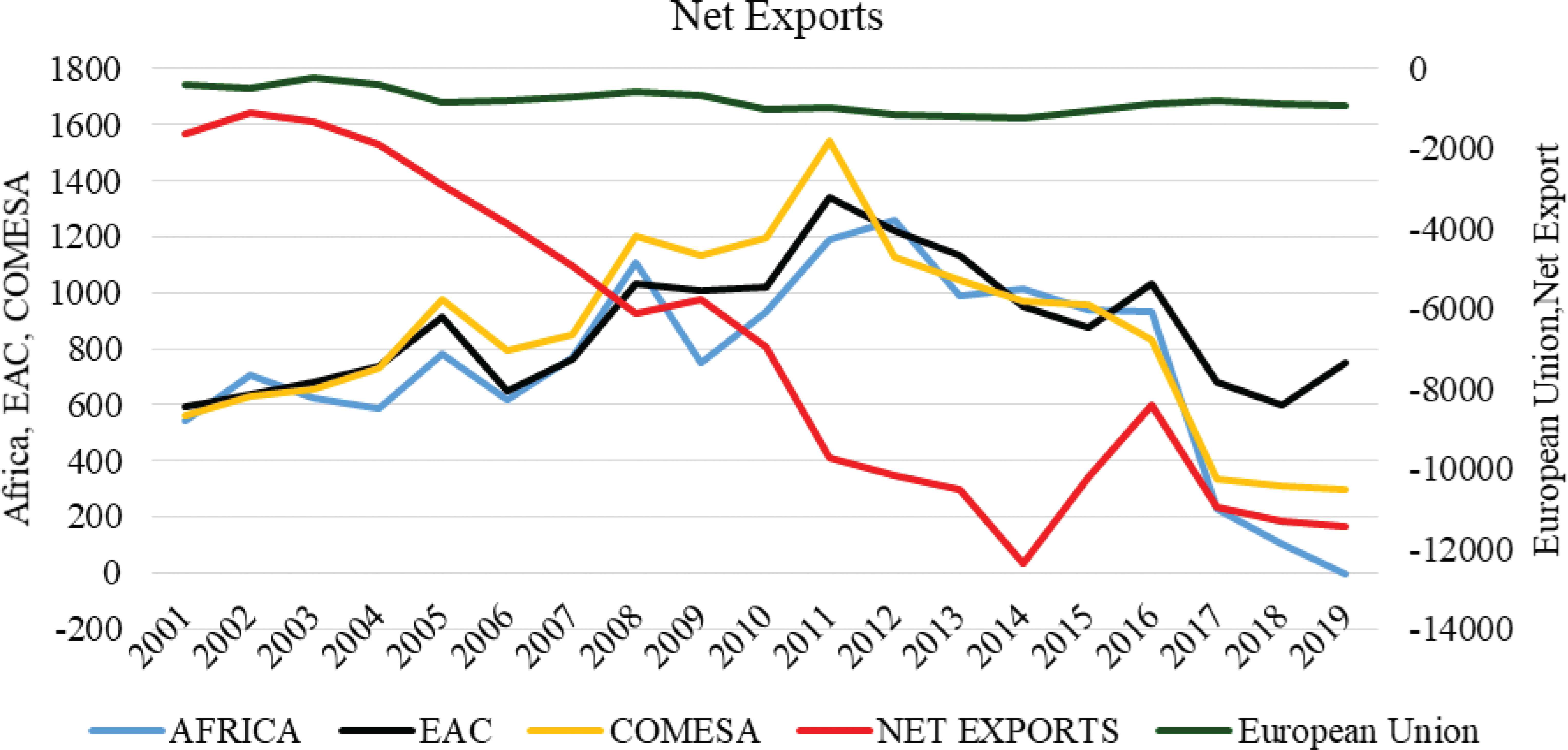
Kenya’s export competitiveness. Source: Authors’ illustration based on CBK data (CBK, 2020).
The loss of export competitiveness and the poor export performance relative to imports widens the trade gap and drags economic growth. The contribution of net exports to real GDP growth has mostly been negative or negligible. Net exports dragged real GDP growth by an average of 1.4% points between 2007 and 2019 due to faster growth of imports, which is a leakage from the economy, unlike exports (Figure 6). Hence, economic growth has largely been sustained by domestic consumption.

Contribution to real GDP growth, by component. Source: Authors’ illustration based on Kenya National Bureau of Statistics data (KNBS, 2019).
3. OVERVIEW OF THE EMPIRICAL LITERATURE ON EXPORTS AND ECONOMIC GROWTH
Empirical studies that attempt to explain the relationship between exports and economic growth are incoherent in terms of findings. For instance, surveys of empirical evidence on the effect of export on economic growth by Giles and Williams (2000) and Awokuse (2007) either establish a positive, no effect, or negative correlation between exports and output growth. In developed countries, Ramos (2001) used a cointegration technique on Portugal data from 1865 to 1998 to test for the long-run relationship between exports, imports, and output growth. The results indicated that output growth leads to growth in exports and imports, but there was no evidence for exports influencing growth in imports. In a related study, Pistoresi and Rinaldi (2012) examined Italy’s trade and economic growth nexus from 1863 to 2004. They established that an increase in intra-industry trade creates bidirectional causality between exports and imports. There was also evidence that imports provide an avenue through which technology is transfused in the economy, while intra-industry trade facilitates technology spillovers. This improves productivity in the export sector and the overall economy, which leads to long-run output growth. Hence, there was evidence for ILG.
Recent studies in developing and emerging economies are also inconclusive. For instance, Pacheco-López’s (2005) analysis of the effects of trade liberalization on economic growth found that it increased imports faster than exports. As a result, an increase in the economy’s productive capacity was stifled due to an increase in consumer imports, and the resultant trade gap constrained economic growth. In addition, Pacheco-López (2005) showed that the Mexican economy experienced stronger output growth during an IS regime than during trade liberalization. Contrary to Pacheco-López (2005), Siliverstovs and Herzer (2006) and Reza et al. (2019) found that manufacturing exports affected output growth, which in turn led to growth in primary exports in Chile. Therefore, there was evidence for ELG with respect to manufactured exports. Lardy (1995) established that foreign trade hastened China’s economic transformation through foreign direct investment and technological progress.
Empirical studies on Africa and Kenya have focused on either the effect of trade openness on growth or exports on growth. For example, Were (2015) investigated the effect of trade openness on growth in developed, developing, and less-developed countries and established that trade positively affects growth in developed and developing countries, but not in least-developed countries. Fosu (1990) found that export growth influenced economic growth positively, based on a sample of 28 less-developed countries in Africa, while Onafowora and Owoye (1998) found evidence in support of ELG using a sample of 12 sub-Saharan African countries. Focusing on Kenya, Kinuthia (2016), using firm-level data, found that exporting firms generate technological spillovers through a demonstration effect and competition, which affects long-run growth within and between industries. On the contrary, Musila and Yiheyis (2015) found that trade is negatively related to growth, while Mwangi et al. (2020) established that agricultural imports are positively related to growth.
The link between exports and growth is not necessarily unidirectional. For example, Siliverstovs and Herzer (2006) and Yang (2008) establish that exports influence growth, while Tang (2006) shows that growth leads to export expansion. The impact of growth on export expansion emanates from the structural changes that growth induces in the economy, which stimulates productivity gains that improve the competitiveness of exports in the international markets (Helpman and Krugman, 1985; Giles and Williams, 2000; Mazumdar, 2001; Awokuse, 2007). Rapid economic growth hastens the rate of technological diffusion. Consequently, the economy can effectively utilize its resources to produce goods and services competitively for the domestic and export markets (Bhagwati, 1989; Hausmann et al., 2007). In addition to growth impacting exports, imports can also influence export growth, which hastens economic growth. Mazumdar (2001) and Hausmann et al. (2007) show that imported capital goods and foreign technology increase the competitiveness of exports and, hence, the volume of exports. Therefore, there is arguably a nexus between exports, imports, and economic growth.
This paper enriches the literature on exports and growth by providing new empirical country evidence, taking into account the endogeneity between exports, imports, and output growth as well as productivity externality generated as a result of international trade and output growth.
4. THEORETICAL FRAMEWORK
The relationship between economic growth and exports can be abstracted from a neoclassical aggregate production function in which technology, capital, and labor are inputs. Exports influence output as they increase the level of technical progress and the quantity of capital. Increasing the level of exports, in particular, increases foreign exchange earnings that are used to import capital goods with advanced technology (Grossman and Helpman, 1990; Mazumdar, 2001). In this regard, exports augment the level of capital stock and accelerate technical progress, which influences long-run economic growth. Competition in the export market compels exporting firms to be innovative so that their products can be competitive. Innovation among exporting firms can be adopted by non-exporting firms and firms in the non-tradable sector. The technological spillovers augment total factor productivity in the aggregate production function (Grossman and Helpman, 1990, 1991; Hausmann et al., 2007). Hence, exporting facilitates technology transfer to firms in the non-export sector and to sectors of the economy with less technological endowment, which increases efficiency. Indeed, total factor productivity in the endogenous growth model enables an economy to produce under increasing returns to scale and realize comparative advantage beyond natural resource endowment.
A combination of high factor productivity and innovation increases competitiveness and improves value addition (Grossman and Helpman, 1990, 1991; Hausmann et al., 2007). In addition, diversification of exports enhances the diversity of innovations, learning, and adoption of a wide range of technologies, which spill over to the economy (Herzer and Nowak-Lehnmann, 2006).
Aggregate output Y consists of domestic production for non-export (N) and export (X) sectors, produced using capital K, labor L, and imported intermediate inputs M. Hence, aggregate production is given by Y = Af(K, L, M), where A is technology. The non-export sector utilizes capital KN, labor LN, and imported intermediate goods MN. In addition, the exporting sector augments productivity in the non-export sector through technological spillovers, which are proportional to the volume of exports. Hence, non-export and export production functions can be specified as N = φX[H(KN, LN, MN)] and X = G(MX, KX, LX), respectively.4 In this specification, exports enter the aggregate production function directly through technological progress and indirectly by easing the foreign exchange constraint that allows the acquisition of intermediate imports (Mazumdar, 2001).
Whereas the externality effect of exports may equalize productivity across the export and non-exporting sectors, export promotion strategies may create productivity differentials. In addition, exporting sectors are more innovative due to exposure to competition and risks in the export market. As a result, productivity differences may exist between the export and non-exporting sectors, influencing output growth. Let HKN, HLN, GKX, and GLX be the marginal productivity of capital and labor in the non-export and export sectors, respectively, then the differential productivity can be denoted as:
Differentiating respective production functions with respect to time yields (small letters represent growth rates):
From Equations (2) and (3), changes in the export growth rate can be accounted for by taking changes in the growth rate of factor inputs in the export production function.
Aggregating export and non-export growth to account for output growth yields:
Finally, collecting like terms and taking the growth rate of capital K over time to be investment I, the output growth equation below is obtained.
From Equation (8), output growth is accounted for by productivity differences in the export sector and externality from the export sector to the rest of the economy, as well as labor, growth in imported intermediate goods, and increase in investment. With regard to the latter, while trade allows a flow of foreign capital into the economy, it reduces the risk of expropriation of private investment. This increases investment in the economy, which in the context of endogenous growth, together with technology, sustains long-run output growth (Rebelo, 1991; Romer, 1986).
5. EMPIRICAL MODEL AND DATA
From the output growth Equation (8), a reduced form production function can generally be specified as follows:
Equation (9) is not easily estimable since it contains indicators of competitiveness (productivity differentials δ across sectors and export productivity externalities φ) which are difficult to measure. However, changes in competitiveness resulting from productivity gains from export externalities can be measured by using a proxy for productivity. Another modification to Equation (8) is the inclusion of life expectancy at birth to control for human capital development Φ. Therefore, the resultant empirical model is specified as follows, in terms of observable and estimable variables:
The empirical model specified by Equation (10) is a standard specification in the endogenous growth and trade literature, and is consistent with Grossman and Helpman’s (1991) and Yang’s (2008) analyses of output growth. The real GDP growth rate is a proxy for output in the growth model. The gross fixed capital formation represents physical capital accumulation in the economy, while labor force growth is the population growth in the productive ages between 15 and 65. Exports, as well as the extent of export diversification, are included sequentially to test for the ELG hypothesis. An increase in exports has the dual effect of generating income leading to enhanced purchasing power for domestic goods and productivity improvement (Grossman and Helpman, 1991). Developing economies import capital goods and technology to increase production capacity and efficiency for domestic consumption and the export market. The externalities generated by imports depend on the diversity of imported goods. Thus, imports and the extent of import diversification are included to test the import-led hypothesis (Yang, 2008). The export and import diversification indices are computed using the Hirschman-Herfindahl index of commodity exports and imports based on the Standard International Trade Classification (SITC).5
Relative changes in factor productivity underpin either ELG or growth-led exports. Improvement in productivity through learning-by-doing and acquiring imported capital goods increases output without necessarily increasing the quantity of inputs. Hence, we include neutral technological progress to capture the productivity gains from growth and international trade (Grossman and Helpman, 1991; Lucas, 1988). Total factor productivity is obtained by undertaking a Hicks decomposition of the constant returns to scale production function.
According to Helpman and Krugman (1985), De Gregorio et al. (1994), and Yang (2008), productivity gains in the tradable sector, firstly, improve the competitiveness of exports in the world market, thereby increasing foreign exchange inflow. Secondly, it either reduces or slows down domestic inflation relative to foreign inflation. As a result, the real exchange rate appreciates. Imports induce real exchange rate depreciation initially through nominal exchange rate depreciation and the increase in prices of imports for final and intermediate use. Imported capital goods increase the productivity of the non-tradable sector, which increases returns to factor payments engaged in the sector. This augments the propensity to spend on consumer imports, which leads to a nominal depreciation (Lucas, 1988; Grossman and Helpman, 1991). As a result, real depreciation due to nominal depreciation and an increase in domestic price relative to foreign price reflect an increase in demand for imports as well as an increase in productivity of the non-tradable sector due to the utilization of imported inputs. Therefore, whereas the real exchange rate can be used as a proxy for productivity, the sign of its coefficient can distinguish productivity gains from either exports or imports (Harberger, 1998; Yang, 2008).6 Hence, we use the real exchange rate to check for the robustness of productivity gains resulting from exports. While depreciation increases the competitiveness of exports, it increases the price of imports which, for import-dependent economies, could lead to increased costs of inputs. Thus, the impact on output depends on the net effect.
For robustness and a much richer analysis, Equation (10) is also estimated at the sectoral output level: agriculture, manufacturing, and services sectors. Analyzing the effect of exports on sectoral output is motivated by the fact that exports may have differential effects on the sectors, masked by aggregation. Moreover, different sectors have different propensities to produce for export and domestic consumption. Further analysis is also conducted by disaggregating exports and imports as well as analyzing the effects of the diversification of imports and exports on growth.
Data for exports, imports, output, labor force, and capital formation covering the period 1960 to 2019 were obtained from the World Development Indicators (World Bank, 2019), while total factor productivity was obtained from the World Productivity database (UNIDO, 2007).7 Commodity exports and imports were obtained from the United Nations Comtrade database (UN COMTRADE, 2019). The advantage of these databases is that they are harmonized, and the series is amenable to long-run analysis.
5.1. Methodology
Estimating Equation (10) poses two challenges. Firstly, most macroeconomic variables tend to be time dependent, a phenomenon that can lead to spurious regression. Secondly, explanatory variables are potentially endogenous. Therefore, estimating such a model by ordinary least squares yields inefficient and inconsistent parameter estimates, compromising the estimates’ validity and the hypothesis testing procedure.
The basic method of assessing the endogeneity status of a variable is the Granger causality test (Granger, 2001). However, the more recent powerful test for causality is the Granger causality/Block exogeneity Wald test (Enders, 2008). By evaluating whether lags of one variable Granger causes other variables,8 the test becomes essential in specifying the Vector Auto-Regression (VAR) model and Vector Error Correction Model (VECM).
The short- and long-run equilibrium relationships between exports, imports, and output in Equation (10) can be estimated by fitting a VECM if the variables are integrated of the same order (Engle and Granger, 1991). However, the existence of variables of a different order of integration necessitates the estimation of a cointegrated Autoregressive Distributed Lag (ARDL) model using the Bounds testing procedure (Pesaran et al., 2001). The VECM and ARDL models provide parameters and error correction terms that suggest how the equilibrium between output and exports is related in the short and long run. VECM can be represented as follows:9
6. EMPIRICAL RESULTS
6.1. Granger Causality and Parameter Estimates
The results of the Granger causality test for the variables are presented in Table A1 in the Appendix. The causality test indicates that exports influence output, while output does not influence exports. There is also a unidirectional effect from exports to productivity. Even though imports affect output, they do not affect productivity. As much as causality is implied, the relationship is not controlled for other explanatory variables, which is a key limitation of the Granger causality test.10 Hence, the need to estimate the long- and short-run relationship between output and exports using the VECM.
Johansen’s cointegration test indicates three cointegrating relationships in Equation (10) (Appendix Table A2). Therefore, there is a long-run relationship between the variables in the output equation, but there are no a priori criteria to identify the three cointegrating relationships. However, plausible long-run equilibrium exists between output, exports, and imports. Exports are used to finance imports. However, the importation of capital and intermediate goods augments the capacity of the economy to produce goods and services for the domestic and foreign markets. Hence, a long-run relationship exists between output, imports, and exports for sustainable growth. The long- and short-run parameter estimates for the three cointegrating relationships from the VECM are presented in Table 1. For brevity, the error correction terms (adjustment coefficients) are reported separately in Table 2.
| ∆OUTPUT | ∆EXPORTS | ∆IMPORTS | |
|---|---|---|---|
| 1 | 2 | 3 | |
| Long-run parameters | |||
| OUTPUT (−1) | 0.799*** [0.249] | 0.174 [0.315] | 0.340 [0.372] |
| IMPORTS (−1) | 0.834*** [0.290] | 0.262 [0.363] | 0.569* [0.438] |
| EXPORTS (−1) | −0.180 [0.131] | 0.135 [0.156] | 0.341 [0.180] |
| Productivity (−1) | 5.956*** [0.761] | 9.047*** [1.684] | 6.379*** [1.577] |
| GFCF (−1) | 0.634*** [0.126] | 1.495*** [0.277] | 1.461** [0.260] |
| HCF (−1) | 3.784*** [0.126] | −0.638 [1.504] | 1.101 [1.408] |
| Short-run parameters | |||
| ∆OUTPUT (−1) | 0.418*** [0.186] | 0.063 [0.269] | 0.293 [0.267] |
| ∆EXPORTS (−1) | 0.329 [0.189] | 0.168 [0.228] | 0.362 [0.269] |
| ∆IMPORTS (−1) | −0.538** [0.234] | −0.500* [0.300] | −0.227 [0.324] |
| ∆Productivity (−1) | 0.360 [0.419] | 0.645* [0.525] | −0.295 [0.620] |
| ∆GFCF (−1) | 0.247* [0.097] | 0.087 [0.117] | 0.128 [0.139] |
| ∆HCF (−1) | 1.225 [2.153] | 4.163*** [2.331] | −0.608*** [2.331)] |
| Exogenous variable | |||
| Labor | 2.120** [0.968] | 0.727*** [0.116] | −0.061*** [0.116)] |
| Constant | −34.244 [15.68] | 11.716*** [1.873] | 1.037 [2.213] |
Notes: OUTPUT is the real GDP, productivity is total factor productivity obtained based on Hicks decomposition of the production function, GFCF is gross fixed capital formation, HCF is the human capital formation proxied by life expectancy at birth. IMPORTS and EXPORTS are total imports and exports, respectively, while Labor is the population in the productive age between 15 and 65. The variables are logs. The ∆ denotes the variable is differenced once, while (−1) indicates that the variable is lagged once, and [..] are standard errors.
*10% **5% ***1% denote levels of statistical significance.
Long- and short-run parameter estimates
| Output | Exports | Imports | |
|---|---|---|---|
| ∆Output | −0.532** [0.235] | −0.047 [0.125] | 0.577* [0.304] |
| ∆Exports | 0.032 [0.268] | −0.053 [0.142] | −0.074 [0.346] |
| ∆Imports | 0.477* [0.312] | 0.375** [0.165] | −0.809** [0.403] |
| ∆Productivity | −0.003 [0.098] | 0.021 [0.052] | 0.019 [0.127] |
| ∆GFCF | 0.586* [0.367] | 0.521** [0.194] | −0.896* [0.473] |
| ∆HCF | 0.007* [0.003] | −0.006*** [0.002] | 0.004 [0.004] |
Notes: Output is the real GDP, productivity is total factor productivity, GFCF is gross fixed capital formation, HCF is the human capital formation proxied by life expectancy at birth. Imports and Exports are total imports and exports, respectively, while Labor is the population between 15 and 65. The variables are logs. The ∆ denotes the variable is differenced, while (−1) indicates that the variable is lagged once, and [..] are standard errors.
*10% **5% ***1% denote levels of statistical significance.
Source: Authors’ analysis.
Error correction coefficients
The results in Table 1, Column 1 show long- and short-run parameter estimates for the output equation. The results show a positive significant long-run relationship between output, imports, total factor productivity, and fixed and human capital formation as proxied by life expectancy. The long-run coefficient of exports in the output equation is negative and statistically insignificant. In the short run, exports have a statistically insignificant positive impact on output, while imports have a negative impact. Column 2 shows that exports are positively influenced by total productivity and fixed capital formation. The short-run impact of human capital formation is also positive. Column 3 shows the long- and short-run parameter estimates for the imports equation. In the long run, imports in the last period, total productivity, and fixed capital formation increase imports in the current period. In contrast, in the short run, exports and output have no statistically significant impact on imports.
The speed of adjustment to long-run equilibrium in the cointegrating relationship between variables in the three cointegrating equations is indicated by error correction coefficients in Table 2. The adjustment coefficient in the output equation, which is fairly large, shows that 53.2% of the deviations of output from the long-run equilibrium are restored or corrected in the same period. Imports correct 47.7% of the deviations in output from the long-run equilibrium, while exports have no statistically significant impact on correcting disequilibrium in output.
The positive adjustment coefficient for imports in the output equation implies that if imports are higher relative to output in the previous period, the output would have to rise in the current period to correct the disequilibrium error of the previous period. This is important for convergence to hold (Enders, 2008). Gross fixed capital formation adjusts 58.6% of short-term disequilibrium in output toward long-run equilibrium in the same period. Human capital formation has a minimal effect on the output adjustment toward the long-run equilibrium. The impact of total factor productivity on output adjustment in the short run is statistically insignificant. Therefore, changes in imports and physical capital formation account for most of the fluctuations in the output growth rate. These results are consistent with the prediction of the endogenous growth models of Romer (1989) and Grossman and Helpman (1990), in which capital formation and technical progress triggered by trade sustain long-run growth.
With respect to the export equation, imports and fixed capital formation correct about 37.5% and 52.1% of export deviations from long-run equilibrium in one year, respectively. In comparison, productivity corrects only 2.1% of the disequilibrium in exports. However, the latter is not statistically significant. A possible channel through which imports influence exports is through imported intermediate and capital goods that have embedded advanced technologies, which augment the competitiveness of exports and efficiency of the sector. Furthermore, physical capital accumulation also promotes export growth as it complements the productive capacity of human capital. The labour coefficient is also positive and statistically significant. This is consistent with the view that commodity exports in Kenya, as in many developing countries, consist of mainly agricultural products that are intensive in unskilled labour, and less competitive in the world market.
The imports equation has comparatively higher speeds of adjustment with respect to correction of disequilibrium resulting from imports, output, and capital formation in the previous period. Changes in output correct 57.7% of the disequilibrium in imports, while imports and fixed capital formation correct 80.9% and 89.6% of the deviation in imports, respectively. The positive effect of output in the imports equation is not surprising, given the relatively high import elasticity with respect to output. Higher output growth increases the propensity to import for consumption and utilization of intermediate or advanced capital goods. It seems relatively easier for the growth in the economy to induce higher import demand than stimulation of exports. The insignificant impact of exports on imports implies that export earnings are insufficient to finance imports.
In general, the results show that changes in output have a stronger effect in stimulating imports and vice versa, relative to exports. Furthermore, short-run deviations in imports from the long-run equilibrium positively and significantly influence export growth. Kenya, like most developing economies, is heavily dependent on imported intermediate and capital goods. Higher national income induces higher growth in imports relative to exports. In particular, the importation of intermediate and capital goods diffuses new technologies in the economy, enhancing production efficiency and increasing output. Thus, there is evidence for ILG.
On the other hand, the adjustment coefficient for exports in both the output and imports equations is statistically insignificant, which suggests that ELG is elusive. These results are consistent with Kenya and other developing economies in which imports are substantially financed by foreign borrowing, aid or grants rather than exports (Esfahani, 1991). In general, the results imply that imports have a greater impact on output and export growth than exports. However, the question is whether such growth is transformative and desirable for job creation, given that imports are a form of leakage with stronger linkages out of the domestic economy.
For robustness, we estimated the empirical model [Equation (10)] using real exchange rate instead of total factor productivity obtained from Hicks decomposition of the production function. The VECM estimates are presented in Table A3 in the Appendix. The long-run coefficients are quantitatively close to those in Table 1. The adjustment coefficients in the output equation indicate that output corrects 1.4% of the deviations of output from the long-run equilibrium in the same period. Imports correct 2.9% of the deviations in output from the long-run equilibrium, but exports do not significantly influence the correction of disequilibrium in output. The real exchange rate adjusts 50% of short-term disequilibrium in output toward long-run equilibrium in the same period. Human capital formation has a small effect on the output adjustment toward the long-run equilibrium. These results are consistent with the findings obtained in Table 1.
The impact of exports and imports on output growth is further assessed by estimating an ARDL model11 using export and import diversification indices instead of exports and imports [Equation (12)]. The Hirschman-Herfindahl indices are used to measure the extent of diversity in imports and exports. In the long run, an increase in export diversification by one point increases output growth by 0.5 percentage points [Equation (12)]. Arguably, the diversification of exports reduces volatility in export earnings and enhances incomes, increasing the propensity to invest and consume, thus acting as a catalyst to economic growth. Producing and exporting a wide range of products also increases the variety of innovations and learning of new and efficient technologies, which spill over to other sectors of the economy (de Piñeres and Ferrantino, 2000).
Notes: Y is the real GDP, PRODUCTIVITY is total factor productivity, GFCF is gross fixed capital formation, and HCF is the human capital formation proxied by life expectancy at birth. IMPORTSCONC and EXPORTSCONC are import and export Hirschman-Herfindahl indices, respectively. Labor is the population between the ages of 15 and 65. The variables are logs. The ∆ denotes the variable is differenced, while (−1) indicates that the variable is lagged once, and [..] are standard errors. *10%, **5%, ***1% denote levels of statistical significance.
Source: Authors’ analysis.
The error correction terms for Equation (12) indicate that diversification of imports and exports corrects about 38.3% and 17.0% of disequilibrium in output, respectively. Hence, diversification of imports has a more profound impact on output growth than that of exports.
6.2. Sectoral Analysis: Exports and Sectoral Output Growth
Table 3 presents VECM estimates based on aggregate exports and sectoral output for the agriculture, manufacturing, and service sectors. The disaggregation allows the analysis of differential effects of exports on different sectors that are likely to be concealed by analysis at the aggregate level. Moreover, some sectors may be more export-oriented than others.
| A | B | C | ||||
|---|---|---|---|---|---|---|
| ∆Agr | ∆Exports | ∆Manufacturing | ∆Exports | ∆Service | ∆Exports | |
| 1 | 2 | 4 | 5 | 6 | 7 | |
| Long-run parameters | ||||||
| Agr (−1) | −0.492 [0.330] | 0.442 [0.322] | – | – | – | – |
| Manufacturing (−1) | – | – | −1.187*** [0.322] | 0.357* [0.213] | – | – |
| Services (−1) | – | – | – | – | 0.585*** [0.182] | −4.591** [2.221] |
| Exports (−1) | −0.224 [0.187] | 0.094 [0.178] | −0.012 [0.313] | 0.132 [0.273] | −0.405** [0.085] | −0.217** [0.107] |
| Imports (−1) | 0.744*** [0.059] | 1.422*** [0.093] | 0.807*** [0.103] | 1.649*** [0.137] | 0.716*** [0.102] | 1.331*** [0.058] |
| Productivity (−1) | 0.431 [0.373] | 2.985*** [0.589] | 0.229 [0.546] | 3.880*** [0.722] | 2.920*** [0.681] | 4.044*** [0.387] |
| GFCF (−1) | 0.218*** [0.054] | 0.299*** [0.085] | 0.190* [0.098] | −0.311** [0.129] | 0.468*** [0.096] | 0.477*** [0.055] |
| HCF (−1) | 4.610*** [1.058] | −5.692*** [1.671] | 0.644 [1.056] | −5.682*** [1.396] | 3.215** [1.804] | 2.074** [1.024] |
| Trend | 0.012 [0.009] | 0.022* [0.014] | – | – | – | – |
| C | – | – | 3.228 | −8.001 | −0.095*** [0.017] | −0.022** [0.009] |
| Error correction coefficients | ||||||
| ∆Agr | −0.510* [0.338] | −0.030 [0.233] | – | – | – | – |
| ∆Manufacturing | – | – | −1.242*** [0.227] | 0.313*** [0.108] | – | – |
| ∆Services | – | – | – | – | −0.614*** [0.185] | 0.293* [0.200] |
| ∆Exports | 0.494 [0.326] | 0.619*** [0.224] | −0.408* [0.218] | 0.224** [0.104] | −0.196 [0.244] | 0.303 [0.264] |
| ∆Imports | 0.794** [0.392] | 0.903*** [0.269] | −0.656** [0.269] | 0.232* [0.129] | −0.657** [0.304] | 0.463 [0.328] |
| ∆Productivity | −0.507** [0.222] | −0.446** [0.158] | 0.028 [0.089] | −0.018 [0.043] | −0.053 [0.049] | −0.496** [0.053] |
| ∆GFCF | −0.720 [0.510] | −0.244 [0.351] | −0.293 [0.347] | 0.023 [0.166] | −1.269*** [0.268] | 0.947** [0.289] |
| ∆HCF | 0.003** [0.001] | 0.001* [0.000] | −0.001 [0.001] | −0.002*** [0.000] | −0.001** [0.001] | 0.000 [0.001] |
| Exogenous variable | ||||||
| Labor | 2.478* [1.471] | 2.788* [1.417] | 3.655** [0.866] | 1.920** [0.833] | −4.637 [2.225] | −0.345 [2.935] |
Notes: Columns A, B, and C present results for the agriculture, manufacturing, and services sectors’ output with the corresponding export cointegrating equation. Agr, manufacturing, and services denote agriculture, manufacturing, and services output, respectively. Imports and Exports are aggregate imports and exports, respectively. GFCF is gross fixed capital formation, HCF is the human capital formation proxied by life expectancy at birth. Labor is the population between the ages of 15 and 65. The variables are logs. The ∆ denotes the variable is differenced once, while (−1) indicates that the variable is lagged once, and [..] are standard errors.
*10% **5% ***1% denote levels of statistical significance.
Source: Authors’ analysis.
VECM results for sectoral output and exports
The results for the sectoral output for the agriculture, manufacturing, and services sectors are presented in Columns A, B, and C in Table 3, respectively. There are two cointegrating vectors for agriculture and services and three for manufacturing output. The short-run coefficients are presented in Table A4 in the Appendix. Column A of Table 3 shows the long-run and error correction coefficients for the agricultural output equation. The results show a positive and significant long-run relationship between agricultural output, imports, fixed capital, and human capital formation. The adjustment coefficients in the agricultural output cointegrating equation indicate that imports, total factor productivity growth, and human capital formation have a statistically significant contribution in correcting the deviation of agricultural output from long-run equilibrium. Changes in fixed capital investment and exports have no statistically significant effect on disequilibrium in agricultural output. Moreover, agricultural output has no statistically significant impact on exports in the long run and short run. The export cointegrating equation’s error correction coefficients indicate that imports, total factor productivity, and human capital formation influence exports. However, the magnitude of the adjustment coefficient for imports is bigger, while the one for human capital formation is negligible.
The results imply that the agricultural output growth is influenced by imports, total factor productivity growth, and capital formation. This is consistent with the finding that imports increase the productivity of the agricultural sector while employing labor, which is then trained to increase skills and boost the growth of the agricultural output in developing economies (Admassie, 2002; Santos-Paulino and Thirlwall, 2004). Most commercial agriculture relies on imported inputs and capital goods such as fertilizer and machinery. However, the impact of exporting on agricultural output is statistically insignificant, even though agricultural output comprises a significant proportion of Kenya’s GDP and exports. This result also gives credence to the slow economic structural transformation and growth in economies that predominantly export primary commodities (UNCTAD, 2017).
In the long run, the manufacturing value-added output is influenced by imports and physical capital formation. Exports are positively impacted by an increase in manufacturing output, imports, and total factor productivity. A 1% increase in the manufactured output in the previous period is associated with a 0.35% increase in current aggregate exports. However, imports have the most significant impact on exports in the long run, with a coefficient of 1.65. In the short run, an increase in manufacturing output by 1% increases exports by 0.23% (Table A4). The adjustment coefficients in Table 3 indicate that imports and exports correct about 65.6% and 41% of the short-run disequilibrium in manufacturing output, respectively. In addition, the adjustment toward long-run equilibrium in the manufacturing sector due to imports is faster than exports. In Kenya, most of the production in the manufacturing sector relies on imported intermediate and capital goods.
In the long run services’ output is positively influenced by imports, total productivity, gross fixed capital formation and human capital development. With regard to the error correction results, changes in imports and fixed capital formation account for the largest adjustments toward long-run equilibrium, while exports have no significant effect. The error correction coefficients indicate that services, total productivity, and physical capital formation correct disequilibrium in exports. The cointegrating equation for exports shows that in the long run, exports are positively associated with imports, total productivity, and investment in physical and human capital and negatively with services sector output. The production of services generates productivity gains, augmented by physical capital to improve export competitiveness in the short and long run. However, in the long run, negative sentiments or instability drags growth in services exports, especially tourism, given the sector’s sensitivity.
Overall, the short-run VECM estimates for sectoral value-added output indicate that imports influence exports, agricultural, manufacturing, and services output. Furthermore, capital accumulation and productivity growth are the main channels through which imports influence sectoral output. Hence, there is evidence for ILG across the sectors in the long run. The results are consistent with the aggregate output analysis, where imports are the primary catalyst of economic growth.
In addition to disaggregating output in the sectors, further analysis was undertaken using disaggregated commodity exports and imports based on SITC classification. The results are presented in Table A5 in the Appendix. Imported manufactured and agricultural commodities have a positive impact on output in the long run. In the short run, manufactured imports positively impact output, while the impact of imported agricultural goods and machinery is negative. Machinery imports also have a negative impact on output in the long run. This indicates that imported machinery and agricultural goods stifle domestic production in the long and short run, respectively.12 However, machinery exports positively impact output in the long run and the short run. The adjustment coefficients in the lower panel of Table A5 show that manufactured exports account for a larger adjustment of output toward its long-run equilibrium compared to manufactured imports. In contrast, agricultural imports have a greater effect on output compared to agricultural exports. The latter reflects the significant role of agriculture in the economy, which relies on imported agricultural inputs. Whereas machinery exports do not significantly influence adjustment of output towards equilibrium, agricultural and machinery imports influence output as well as exports of other machinery. The positive impact of agricultural imports on output is also established by Mwangi et al. (2020). The results generally provide further evidence that exports have a small effect on growth compared to imports. In addition, results indicate that manufactured imports generate more considerable growth-enhancing externalities than primary imports.
7. CONCLUSION
This paper examines the relationship between exports, imports, and growth in Kenya in the context of endogenous growth models. Although Kenya has liberalized international trade and implemented policies to diversify and promote exports, the country’s export growth has been sluggish, and predominantly consists of primary agricultural commodities such as tea, coffee, and horticulture. Empirical evidence indicates that there is a long-run relationship between exports, imports, and output. However, the impact of exports on output growth is not statistically significant; instead, output growth is largely influenced by imports. In addition, import diversification has a larger impact on output compared with the diversification of exports. Sectoral analysis further shows that imports influence agricultural, manufacturing, and services output. Other determinants of aggregate and sectoral output growth include total factor productivity and capital formation. Furthermore, exports are influenced by growth in imports, manufactured output, and capital formation. Analysis using disaggregated import and export data shows that imported manufactured and agricultural goods positively impact output growth. Nonetheless, the impact of machinery exports on economic growth is also positive. However, in general, long-run output growth seems to be sustained by imports, with higher economic growth acting as a trigger for the growth of imports. Hence, there is more evidence for import-led growth (ILG) than for export-led growth (ELG), notwithstanding the crowding out of domestic production by machinery and agricultural imports in the short run. However, ILG may not be consistent with the country’s strategy of utilizing ELG to achieve structural transformation and development.
Like most developing and low-income African economies, Kenya’s economy is heavily dependent on imported intermediate and capital goods. Arguably, imports contribute to technology transfer to the domestic economy, which enhances productivity and output. However, the export sector does not seem to be competitive enough to significantly influence the transformation of the economy and contribute substantially to robust economic growth. As a result, ELG is still elusive, despite the notable progress in trade liberalization and export promotion.
Notwithstanding the insignificant impact of aggregate exports on economic growth, analysis using disaggregated data implies that increasing diversification of exports toward manufactured and machinery exports, enhancing the value addition of agricultural exports, increasing local content, and adopting new and efficient methods of production in the exporting sector are likely to enhance ELG. This could be achieved by integrating the economy in regional and global value chains. Kenya should leverage on the AfCFTA as one of the avenues for boosting exports in the African region.
CONFLICTS OF INTEREST
The authors declare that they have no conflicts of interest.
AUTHORS’ CONTRIBUTION
PSW and MW contributed in study conceptualization and writing the manuscript. PSW contributed in data curation, empirical analysis while MW reviewed literature and contributed in writing and editing the manuscript. Comments on the original and revised drafts were addressed by both PSW and MW.
FUNDING
The authors did not receive funding to write this paper.
ACKNOWLEDGMENTS
The authors are grateful for the comments by participants of the UNUWIDER Research Seminar held in April 2019 and insightful reviews by Augustin Fosu. The usual disclaimer applies.
APPENDIX
| Null hypothesis | Obs | F-Statistic | Prob. |
|---|---|---|---|
| Exports does not Granger cause output | 54 | 4.095 | 0.023 |
| Output does not Granger cause exports | 0.042 | 0.959 | |
| Imports does not Granger cause output | 54 | 4.757 | 0.013 |
| Output does not Granger cause imports | 1.858 | 0.167 | |
| Productivity does not Granger cause output | 54 | 0.003 | 0.997 |
| Output does not Granger cause productivity | 0.711 | 0.496 | |
| GFCF does not Granger cause output | 54 | 2.484 | 0.094 |
| Output does not Granger cause GFCF | 1.205 | 0.309 | |
| HCF does not Granger cause output | 53 | 0.790 | 0.460 |
| Output does not Granger cause LE | 18.453 | 0.000 | |
| Imports does not Granger cause exports | 54 | 0.451 | 0.64 |
| Exports does not Granger cause imports | 4.189 | 0.021 | |
| Productivity does not Granger cause exports | 54 | 0.257 | 0.774 |
| Exports does not Granger cause productivity | 4.632 | 0.014 | |
| GFCF does not Granger cause exports | 54 | 1.239 | 0.299 |
| Exports does not Granger cause exports | 0.457 | 0.636 | |
| HCF does not Granger cause exports | 53 | 1.313 | 0.279 |
| Exports does not Granger cause HCF | 16.281 | 0.000 | |
| Productivity does not Granger cause imports | 54 | 0.523 | 0.596 |
| Imports does not Granger cause productivity | 1.476 | 0.239 | |
| GFCF does not Granger cause imports | 54 | 2.958 | 0.061 |
| Imports does not Granger cause GFCF | 0.357 | 0.701 | |
| HCF does not Granger cause imports | 53 | 0.807 | 0.452 |
| Imports does not Granger cause HCF | 18.236 | 0.000 | |
| GFCF does not Granger cause productivity | 54 | 2.188 | 0.123 |
| Productivity does not Granger cause GFCF | 0.638 | 0.533 | |
| HCF does not Granger cause productivity | 53 | 0.99 | 0.379 |
| Productivity does not Granger cause HCF | 0.253 | 0.778 | |
| HCF does not Granger cause GFCF | 53 | 0.517 | 0.599 |
| GFCF does not Granger cause HCF | 20.072 | 0.000 | |
Source: Authors’ computations based on World Bank (2019) and UNIDO (2007) data.
Granger causality test
| Hypothesized | ||||
|---|---|---|---|---|
| No. of CE(s) | Eigenvalue | Trace statistic | Critical value 0.05 | Prob. |
| None* | 0.936 | 273.259 | 117.708 | 0.000 |
| At most 1* | 0.693 | 127.504 | 88.804 | 0.000 |
| At most 2* | 0.432 | 64.932 | 63.876 | 0.041 |
| At most 3 | 0.302 | 34.955 | 42.915 | 0.247 |
| At most 4 | 0.152 | 15.907 | 25.872 | 0.500 |
| At most 5 | 0.126 | 7.165 | 12.518 | 0.328 |
Notes: Labor is exogenous. Trace test indicates three cointegrating equation(s) at the 0.01 level.
*Denotes rejection of the hypothesis at the 0.01 level. Max-eigenvalue test indicates two cointegrating equation(s) at the 0.01 level.
Source: Authors’ computations based on World Bank (2019) data.
Cointegration rank test (trace)
| ∆Output | ∆Exports | ∆Imports | |
| 1 | 2 | 3 | |
| Output (−1) | −1.033*** [0.235] | −0.306 [0.303] | 0.149 [0.373] |
| Exports (−1) | −0.226 [0.112] | −0.087 [0.145] | 0.291 [−0.179] |
| Imports (−1) | 1.037*** [0.287] | −0.355 [0.373] | −0.483 [0.458] |
| Productivity (−1) | −1.244*** [0.130] | −1.963*** [0.36] | −1.745*** [0.200] |
| GFCF (−1) | 0.271*** [0.083] | 0.624*** [0.229] | 0.375*** |
| −0.127 | |||
| HCF (−1) | 6.909*** [0.304] | 9.745*** [0.842] | 8.194*** [0.466] |
| C | 18.846*** [1.522] | 14.972*** [4.215] | 19.347*** [2.334] |
| Error correction coefficients | |||
| Output | Exports | Imports | |
| ∆Output | −0.014* [0.011] | 0.056 [0.142] | 0.775*** [0.289] |
| ∆Exports | −0.013 [0.015] | 0.085 [0.190] | 0.219 [0.388] |
| ∆Imports | −0.029* [0.017] | 0.725*** [0.212] | −0.938** [0.432] |
| ∆Productivity | 0.493*** [0.188] | −0.224* [0.119] | −0.138 [0.242] |
| ∆GFCF | 0.483 [0.433] | 0.711*** [0.274] | −1.270*** [0.557] |
| ∆HCF | −0.000*** [0.000] | −0.002 [0.002] | 0.005 [0.003] |
| Exogenous variable | |||
| Labor | 0.492*** | 0.196 | 0.172 |
| [0.115] | [0.154] | −0.293*** | |
Notes: Trace test of VAR model with the real exchange rate as a proxy for productivity indicates three cointegrating vectors. Output is the real GDP, productivity is the real exchange rate, GFCF is gross fixed capital formation, and HCF is life expectancy at birth. Labor is the population between ages 15 and 65. The variables are logs except for the real exchange rate. The imports and exports in Column 4 are Hirschman-Herfindahl indices for commodity exports and imports. The Hirschman-Herfindahl index is used to measure diversity in exports and imports. The ∆ preceding a variable indicates that the variable is differenced once, while (−1) indicates that the variable is lagged once, and [..] are standard errors.
*10% **5% ***1% denote levels of statistical significance.
Source: Authors’ analysis based on World Bank (2019) data.
VECM estimates
| A | B | C | ||||
|---|---|---|---|---|---|---|
| AGRICULTURE | EXPORTS | MANUFACTURING | EXPORTS | SERVICE | EXPORTS | |
| ∆AGR (−1) | 0.366 [0.270] | −0.256 [0.260] | – | – | – | – |
| ∆AGR (−2) | 0.374* [0.225] | −0.052 [0.216] | – | – | – | – |
| ∆Manufacturing (−1) | – | – | 0.606*** [0.187] | 0.230** [0.180] | – | – |
| ∆Manufacturing (−2) | – | – | 0.422*** | 0.090 | – | – |
| −0.167 | −0.161 | |||||
| ∆Service (−1) | – | – | – | – | 0.090 [0.212] | −0.041 [0.279] |
| ∆Service (−2) | – | – | – | – | −0.062 [0.199] | −0.137 [0.263] |
| ∆Exports (−1) | 0.021 [0.329] | −0.528** [0.317] | −0.307* [0.260] | −0.273 [0.250] | −0.066 | −0.196 [0.369] |
| 0.280 | ||||||
| ∆Exports (−2) | −0.166 [0.274] | −0.584** [0.264] | −0.575** [0.251] | −0.451* [0.241] | −0.146 [0.243] | −0.301 [0.320] |
| ∆Imports (−1) | −0.240 [0.415] | 0.805*** [0.400] | −0.195 [0.283] | −0.008 [0.272] | 0.121 [0.287] | 0.091 [0.379] |
| ∆Imports (−2) | 0.203 [0.287] | 0.755*** [0.277] | 0.220 [0.243] | 0.326 [0.234] | 0.394 [0.257] | 0.429 [0.339] |
| ∆Productivity (−1) | −0.071 [0.567] | −1.150*** [0.547] | −1.082*** [0.538] | −0.962** [0.517] | 0.451 [0.742] | −0.496 [0.979] |
| ∆Productivity (−2) | −0.758* [0.492] | −0.297 [0.474] | −0.449 [0.463] | 0.004 [0.445] | 0.363 [0.627] | 0.209 [0.827] |
| ∆GFCF (−1) | 0.172 [0.146] | −0.113 [0.140] | 0.162 [0.124] | 0.015 [0.119] | 0.247 [0.124] | 0.116 [0.164] |
| ∆GFCF (−2) | −0.139 [0.131] | −0.280** [0.126] | 0.035 [0.117] | −0.113 [0.113] | 0.139 [0.114] | −0.070 [0.150] |
| ∆HCF (−1) | 28.544 [20.247] | 32.674 [19.505] | 43.351** [14.065] | 35.308*** [13.519] | 6.443 [46.961] | 44.404 [61.941] |
| ∆HCF (−2) | −27.566 [19.726] | −25.212 [19.003] | −36.219 [12.585] | −29.061** [12.097] | −76.130 [83.869] | −62.312 [110.622] |
| C | −9.657** [5.759] | −10.870** [5.548] | −14.269 [3.394] | −7.461 [3.262] | 18.132 [8.699] | 1.389 [11.474] |
| LABOR | 2.478** [1.471] | 2.788** [1.417] | 3.655*** [0.866] | 1.920*** [0.833] | −4.637 [2.225] | −0.345 [2.935] |
Notes: Columns A, B, and C present short-run coefficients for the agriculture, manufacturing, and services sector output equations and the corresponding cointegrating exports equation. The variables in the equation are Agr (agricultural output), manufacturing sector output, output from the services sector, total factor productivity, GFCF (gross fixed capital formation), and HCF (life expectancy at birth). Labor is the population between ages 15 and 65. The variables are in logs except for total factor productivity. The ∆ preceding a variable indicates that the variable is differenced once, while (−1) indicates that the variable is lagged once, and [..] are standard errors.
*10% **5% ***1% denote levels of statistical significance.
Source: Authors’ analysis based on World Bank (2019) and UNIDO (2007) data.
Short-run parameters
| A | B | C | |||||
| Number of cointegrating vectors | 2 | 2 | 3 | ||||
| Cointegrating Eq: | Output | MANUFEX | Output | AGRICEX | Output | MACHEX | MACHIM |
| MANUFIM (−1) | 0.905*** [0.152] | 1.596*** [0.354] | – | – | – | – | – |
| AGRICEX (−1) | – | – | – | – | – | – | – |
| AGRICIM (−1) | – | – | 0.799*** [0.471] | −0.702*** [0.084] | – | – | – |
| MACHIEX (−1) | – | – | – | – | 0.133*** [0.039] | 0.177 [0.410] | 0.007 [0.134] |
| MACHIM (−1) | – | – | – | – | −0.383* [0.205] | 0.643 [2.147] | −0.721 [0.701] |
| Productivity (−1) | 0.754*** [0.172] | 0.546* [0.401] | 0.328 [1.249] | 1.482*** [0.223] | 0.347 [0.497] | 2.515** [0.632] | −3.998** [0.352] |
| GFCF (−1) | 1.268*** [0.179] | 1.252*** [0.415] | 0.960 | 0.737*** | 1.297** [0.327] | 2.755** [0.416] | −0.590** [0.232] |
| 0.832 | 0.149 | ||||||
| HCF (−1) | 4.711*** [0.413] | 4.345*** [0.960] | 19.930** [6.294] | 8.371*** [1.126] | 4.604 [1.687] | 23.209*** [2.145] | 9.944*** [1.196] |
| Short-run parameters | |||||||
| CointEq1 | CointEq2 | CointEq1 | CointEq2 | CointEq1 | CointEq2 | CointEq3 | |
| ∆Output | 0.278 [0.269] | 0.759 [0.571] | 0.000 [0.462] | −1.126 [1.073] | 0.206 [0.235] | 2.717 [1.072] | −0.001 [0.538] |
| ∆MANUFEX | −0.036 [0.142] | 0.736** [0.302] | – | – | – | – | – |
| ∆MANUFIM | 0.738** [0.204] | −1.001*** [0.434] | – | – | – | – | – |
| ∆AGRICEX | – | – | −0.235** [0.191] | −0.134 [0.445] | – | – | – |
| ∆AGRICIM | – | – | −0.109*** [0.097] | −0.111 [0.226] | – | – | – |
| ∆MACHIEX | – | – | – | – | 0.054* [0.036] | −0.095 [0.165] | 0.071 [0.085] |
| ∆MACHIM | – | – | – | – | −0.186* [0.105] | −0.228 [0.478] | 0.083 [0.240] |
| ∆Productivity | 1.638*** [0.503] | 1.992 [1.068] | −0.324 [0.495] | −1.369 [1.151] | 0.167* [0.304] | 2.964* [1.388] | 0.416 [0.697] |
| ∆GCFC | 0.088 [0.308] | 0.883** [0.655] | 0.091 [0.213] | −0.059 [0.496] | 0.116 [0.158] | 0.020 [0.722] | 0.460* [0.363] |
| ∆HCF | 32.949 [107.993] | 140.624 [229.183] | 63.553 [25.954] | −86.704 [60.362] | 0.284 [1.814] | 24.503*** [8.285] | −0.693 [4.162] |
| Exogenous variable | |||||||
| Labor | −40.301 [10.978] | 90.231 [23.297] | 30.282 [27.707] | 107.847 [64.438] | 0.029 [0.065] | −0.725** [0.295] | −0.035 [0.148] |
| Adjustment coefficients | |||||||
| Cointegrating | Output | MANUFEX | Output | AGRICEX | Output | MACHEX | MACHIM |
| ∆Output | −0.387* [0.288] | −0.703*** [0.157] | −0.050** [0.017] | −0.231 [0.416] | −0.013 [0.062] | 0.067 [0.047] | 0.942** [0.212] |
| ∆MANUFEX | −1.624** [0.610] | 0.045 [0.624] | – | – | – | – | – |
| ∆MANUFIM | 0.436 [0.623] | −0.437 [0.380] | – | – | – | – | – |
| ∆AGRICEX | – | – | 0.041 [0.040] | −0.051* [0.038] | – | – | – |
| ∆AGRICIM | – | – | 0.096*** [0.035] | −0.086*** [0.025] | – | – | – |
| ∆MACHEX | – | – | – | – | 0.795 [2.079] | −0.001 [0.417] | −0.643 [2.324] |
| ∆MACHIM | – | – | – | – | −1.234* [0.941] | 0.080 [0.108] | 0.741* [0.601] |
| ∆Productivity | 0.988*** [0.257] | 0.327** [0.127] | 0.031*** [0.012] | 0.036*** [0.012] | −0.043 [0.048] | −0.102*** [0.036] | −0.592** [0.147] |
| ∆GFCF | −1.073** [0.560] | −0.482* [0.277] | −0.060** [0.020] | −0.058** [0.020] | 0.047 [0.080] | 0.044 [0.060] | 0.054 [0.317] |
| ∆HCF | −0.002* [0.001] | −0.001** [0.000] | 0.000 [0.000] | 0.000 [0.000] | 0.009*** [0.001] | 0.001 [0.001] | 0.001 [0.001] |
Notes: Columns A, B, and C present results for VECM long- and short-run coefficients for manufactured, agriculture, and machinery imports and exports, respectively. The numbers of the respective cointegrating vectors are indicated in row 2. MANUFEX – manufactured export, MANUFIM – manufactured import, AGRICIM –agricultural imports, AGRICEX – agricultural exports, MACHIM – machinery imports, MACHEX – machinery exports, productivity is total factor productivity GFCF – gross fixed capital formation. HCF – Human capital formation, Labor is the population between ages 15 and 65. The variables are in logs except for the real exchange rate. The ∆ preceding variable indicates that the variable is differenced once, while (−1) indicates that the variable is lagged once, and [..] are standard errors.
*10% **5% ***1% denote levels of statistical significance.
Source: Authors’ analysis.
Commodity exports and growth
Footnotes
A sector producing under increasing returns to scale generates efficiency externalities to other sectors. The efficiency externalities augment long-run growth beyond resource endowment.
Launched in 2000, AGOA provides special market access to sub-Saharan African beneficiary countries for the export of a number of products to the USA.
If countries produce import-competing goods, a decline in net exports implies that the competitiveness of domestically produced goods is declining both in the domestic and foreign markets as intra-industry trade intensifies.
Then, the aggregate production function can be specified as: Y = A(X) f (K, L, M).
The diversification index is a Hirschman-Herfindahl index of commodity exports and imports, categorized based on SITC. An increase in the index implies a decline in the diversity of export and import, implying that the economy tends to export and import a narrow range of products.
Productivity improvement in the non-tradable sector increases demand for domestically produced goods as well as imports. The increase in demand for imports leads to a real exchange rate depreciation. Productivity improvement in the tradable sector increases exports. Consequently, the real exchange rate appreciates due to an increase in foreign exchange earnings.
The data on productivity sourced from World Productivity database is based on Hicks neutral production technology. Missing data points for total factor productivity were, therefore, updated using Hicks production function.
The null hypothesis is that all the lags of one variable can be excluded for the equation.
If VAR (p) is given by a vector Zt, then
The Granger causality test does not account for the relative impact of other explanatory variables such as labor, physical capita formation, life expectancy, and imports on growth. As a result, joint contribution of the potential explanatory variables in explaining variation in output is omitted, which bias the results.
GDP, Productivity, GFCF and HCF are integrated of order 1, while EXPORTSCONC and IMPORTSCONC, which is Hirschman-Herfindahl index of diversity, are stationary. Therefore, the equation is estimated using the bound testing procedure (see Pesaran et al., 2001).
The short- and long-run parameters estimated from a cointegrated relationships require may not be unique, which may undermine inference and conclusions. See Greenslade et al. (2002) on identification problem in cointegrating equations.
REFERENCES
Cite this article
TY  - JOUR
AU  - Peter Simiyu Wamalwa
AU  - Maureen Were
PY  - 2021
DA  - 2021/09/07
TI  - Is it Export- or Import-Led Growth? The Case of Kenya
JO  - Journal of African Trade
SP  - 33
EP  - 50
VL  - 8
IS  - 1
SN  - 2214-8523
UR  - https://doi.org/10.2991/jat.k.210818.001
DO  - 10.2991/jat.k.210818.001
ID  - Wamalwa2021
ER  -