
Trade Costs and Demand-Enhancing Effects of Agrifood Standards: Consequences for Sub-Saharan Africa
- DOI
- 10.2991/jat.k.210907.001How to use a DOI?
- Keywords
- Non-tariff measures; sanitary and phytosanitary measures; technical barriers to trade; sub-Saharan Africa; ad valorem equivalent; gravity model
- Abstract
Agrifood standards impede trade by increasing compliance costs, but they can also enhance trade by signalling quality. This paper disentangles the trade costs and demand-enhancing effects of two important standards—technical barriers to trade, and sanitary and phytosanitary measures—on (i) global agricultural trade flows and (ii) fruit, nut, and vegetable trade between sub-Saharan Africa and high-income OECD countries. Combining estimates fromunit value and trade value regressions set within structural gravity frameworks, we show that trading standards increase trade costs—which exporters pass on to consumers in the form of higher prices—but they also increase trade volume. For agrifood exports from sub-Saharan Africa, compliance with standards guarantees market access at higher prices to high-value OECD markets.
- Copyright
- © 2021 African Export-Import Bank. Publishing services by Atlantis Press International B.V.
- Open Access
- This is an open access article distributed under the CC BY-NC 4.0 license (http://creativecommons.org/licenses/by-nc/4.0/).
1. INTRODUCTION
Standard-like non-tariff measures—henceforth, standards or NTMs—have gained prominence as policy instruments to regulate agricultural trade. The current infrequent use of traditional instruments, e.g., tariffs, quotas, and voluntary restraints, only exacerbates their relevance. Their increasing relevance is fuelled by two types of NTMs: sanitary and phytosanitary (SPS) measures, and technical barriers to trade (TBTs). These measures are prima facie introduced to correct market imperfections by alleviating information asymmetry, mitigating food consumption risks, and enhancing sustainability. So while these measures have no explicit trade objective, they can be disguised instruments for protection.
In many high-value markets, export success is now conditioned on compliance with NTMs. Export competition is also shifting from prices to quality (Curzi et al., 2015). Even with zero tariffs, as guaranteed under many preferential trade agreements, exports must pass stringent standards in their destination markets. This is a problem for countries that have limited capacities to meet the regulatory requirements associated with standards, notably the least developed countries (Xiong and Beghin, 2014; Ferro et al., 2015). However, standards are not without advantages when it comes to trade. They can facilitate trade by playing the role of positive demand shifters if they inform buyers that a product meets their expected quality level.1 This facilitates participation in global value chains as compliant firms from developing countries overcome reputational challenges to access high-value markets (Fiankor et al., 2019; World Bank, 2020). Hence, standards can have signalling effects strong enough to increase trade volume even though they imply higher compliance costs. In the end, the standards–trade effect is an empirical question.2 The existing empirical evidence reflects this ambiguity:3 standards enhance (Crivelli and Gröschl, 2016; Shingal et al., 2021), impede (Fiankor et al., 2021a, 2021b), or have no effect (Xiong and Beghin, 2012; Schuster and Maertens, 2015) on trade.
With approximately 70% of all least-developed countries located in sub-Saharan Africa (SSA), the threat (or otherwise) posed by standards to agrifood trade has direct implications for the region. For instance, agricultural exports are a mainstay of the economy in many SSA countries, yet the share of SSA’s agricultural exports in global trade has remained fairly stable over the last two decades (Figure 1a). Over the same period, the share of SSA’s high-value agrifood exports, such as fruits, nuts, and vegetables, has been steadily increasing, from 2.5% in 2001 to 4.5% in 2018. Despite this trend, the share of SSA’s agricultural exports to high-income OECD countries has been decreasing, especially for fruits, nuts, and vegetables (Figure 1b). This is despite the fact that over the last decades, many developing countries have witnessed structural shifts from exporting traditional cash crops to non-traditional high-value agrifood products, including fresh fruits and vegetables (Reardon et al., 2009). This contrast between decreasing exports to the OECD (Figure 1a) and the increasing share of high-value agrifood products in global exports (Figure 1b) raises a policy-relevant question: What are the possible reasons behind this phenomenon? In this study, we investigate empirically the role of standards imposed by high-income OECD countries on high-value fruits and vegetables. For example, 78% of all mangoes intercepted at the EU border in 2016 because of pest infestation were of African origin, and 46% of all interceptions at the EU border because of a failure to show SPS-related certificates were from Africa (Grumiller et al., 2018).
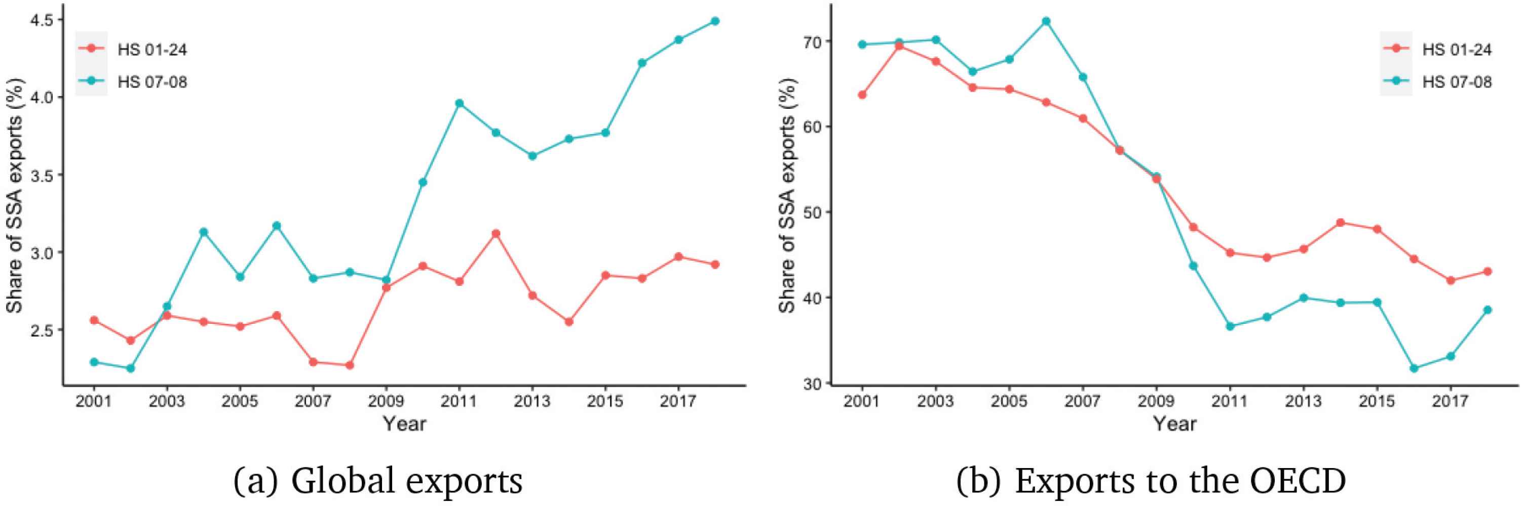
Agricultural trade between OECD countries and SSA—status quo. Source: Trademap data, original graph.
In light of the arguments above, the debate on the relationship between trade and standards is not on the “if”, since there is a clear consensus that they can affect trade, but rather on the “how.” That is, it is unclear to what extent they affect trade (Abbyad and Herman, 2017). To answer the “how” question, the literature resorts to the ad valorem equivalent (AVE) measure.4 However, a focus on only the AVE provides a one-sided story. It is necessary to combine the AVEs with the effect on traded volumes to assess the full effects of NTMs on trade. In this paper, we combine these two mechanisms to disentangle the trade costs and demand-enhancing effects of standards in agricultural trade using HS6 digit product-level data for the period from 2012 to 2016. As a first empirical exercise, we study AVEs for all countries and all agricultural products. We then focus on the trade of edible fruits, nuts, and vegetables between SSA and high-income OECD countries. To estimate the trade-cost effects, we apply a combination of approaches where the AVE is obtained directly from the marginal effect of NTMs on unit values (Cadot and Gourdon, 2016; Ghodsi et al., 2016; Sanjuán et al., 2019). In a second step, we estimate their effects on the volume of trade. We combine the results from both price and quantity estimations to assess the ultimate trade effects of standards for agrifood trade.
To situate our paper in the literature, we begin with trade policy. In general, this work contributes to a relatively under-researched but relevant topic in agricultural trade. Ours is the first effort to disentangle the trade-cost and demand-enhancing effects of NTMs using panel data of bilateral AVE for all agricultural products (HS01–HS24) and countries. Existing research, such as Cadot and Gourdon (2016), uses cross-sectional data and focuses on all products in the HS classification. Closest to our work is Gourdon et al. (2020) who investigate the trade-cost and trade-enhancing effects of SPS and TBT measures, along with other types of NTMs in agricultural trade. However, because they work with data for a single year, ours is the first panel data analysis in the agricultural trade literature. We use a bilateral measure of NTMs, i.e., where applicable, exporter–importer-specific standards, complementing earlier works (e.g., Cadot et al., 2018b; Sanjuán et al., 2019; Gourdon et al., 2020).
Our paper is also related to the literature on the trade effects of technical standards on African exports to the Global North, which is too extensive to be comprehensively summarised here.5 These studies have focused entirely on the standards–trade effects at the intensive margin, i.e., the value of conditional export sales (Otsuki et al., 2001), the extensive margin, i.e., the probability of trade (Kareem et al., 2017, 2018), or a combination of both trade margins (Xiong and Beghin, 2012; Kareem, 2016; Kareem and Rau, 2018). As a result, the existing literature analyses only the trade-enhancing or impeding effects of NTMs, ignoring in large part their trade cost or price effect. Our contribution is to connect these trade and price effects to provide a holistic approach to the standards–trade debate and to offer more targeted conclusions. This is important because price effects may differ depending on the origin of the imports (Sanjuán et al., 2019; Emlinger and Guimbard, 2021), pointing to possible compliance cost differences across exporters.
2. EMPIRICAL APPROACH
To disentangle the effects of standards, we follow closely the conceptual frameworks of Xiong and Beghin (2014)6 and Cadot et al. (2018b), presented in the appendix. Our empirical strategy is to estimate the following sector-level gravity equation of Anderson and Van Wincoop (2004):
Xsijt varies depending on which of the two economic effects, prices (Psijt), or trade volumes (Qsijt) we consider. SPSsijt and TBTsijt are respectively the number of SPS and TBT measures imposed on HS6 digit level product s exported from i to importer j in year t. The superscripts A and B on β1 designate type A (SPS) and type B (TBT) NTMs using UNCTAD classifications. The superscript C designates all other NTM types excluding export measures (Figure A1 in the appendix). Following recent literature (Murina and Nicita, 2017; Cadot et al., 2018b; Sanjuán et al., 2019), our NTM variable is the count of one-letter, three-digit NTMs (A110, B120, etc.) for each category in a trade dyad.7 Following Peci and Sanjuán (2020), our NTM variables are not log transformed. Thus, β1 captures marginal effects and not elasticities. NTMs in general are endogenous to trade volumes (Looi Kee et al., 2009). The reasoning is that the more an agricultural product is imported, the higher the incidence of SPS measures, as policymakers try to safeguard the health of domestic consumers (Murina and Nicita, 2017). The trade and price effects of NTMs may also occur with some delay. Hence, we lag our NTM variables by one period to account for possible reverse causality (Ferro et al., 2015; Niu et al., 2018). Endogeneity due to omitted variables is controlled for using the country- and product-time fixed effects.
Tariffsijt is the applied tariff. The vector G includes traditional time-varying and time-invariant gravity variables, including preferential trade agreements (PTAs), membership of the World Trade Organisation (WTO), bilateral distance, common language, and contiguity. As Anderson and Van Wincoop (2003) show in their seminal paper, relative trade resistance rather than just absolute trade resistance is more appropriate for explaining bilateral trade flows. Following Feenstra (2004), we include year-specific importer (fejt) and exporter (feit) fixed effects to account for these multilateral trade resistance terms. The fixed effects account for observable and unobservable importer- and exporter-specific time-varying variables, such as GDP, population, and quality of domestic institutions. We also include time-varying product fixed effects (fest) to control for any product-specific effects. usijt is an error term which we cluster at the country-pair-product level.
2.1. Price-Based Estimation, Estimating Trade-Cost Effect (AVE)
Taking the log of the equilibrium price (Equation 11 in the appendix) we can empirically estimate the price effect (AVE) as Equation (2). Since we are particularly interested in isolating the effect for SSA exports to high-income OECD countries, we adopt the “route approach”.8 This involves the interaction of the NTM variable with dummies of a given trade route—i.e., one dummy for the origin and another for the destination—to estimate the AVE for this particular trade route. Our first estimation equation is thus the following:
Since zero-value traded products do not have a price—and are excluded from the price equation—we estimate Equation (2) using ordinary least squares (OLS).
2.2. Quantity-Based Estimation, Estimating Demand-Enhancing Effect
To assess the trade effect, we estimate the following equation:
2.3. Equilibrium Changes—Combining Price-Based and Quantity-Based Estimations
If Equations (2) and (3) yield positive and statistically significant β1 coefficients, the observed demand-enhancing effect surpasses the trade-cost effect. The reverse is true when Equation (3) yields negative and significant β1 coefficients. If, however, Equation (2) yields positive and significant β1 estimates while the estimates in Equation (3) are statistically insignificant, then the trade-enhancing and trade-cost effects neutralise each other. When both equations yield statistically insignificant β1 estimates, the standards imposed are ineffective.
3. DATA
The dataset includes global agricultural trade flows (Table A1 of the appendix). This dataset is used for the first part of our empirical analysis. To assess the effects for Africa specifically, our identification strategy in the second part of our empirical analysis exploits data on 44 SSA country exports to 25 OECD countries. GTAP Section 4 (vegetable, fruits, nuts), which corresponds to chapters 7 and 8 in the HS Nomenclature 2012 Edition, is used for this part of the study. The choice of OECD importing countries is based on their income level. We expect that consumer awareness and food safety concerns are relatively higher in these countries and thus may influence policymaking and consumer behaviour. High-income OECD countries are increasingly strict on issues related to product quality and do not accept consignments even with minor variations (Ing et al., 2016). According to the 2020 World Development Report (World Bank, 2020), the higher the income level of a country, the lower the level of tariffs and the more it is likely to make extensive use of standards. This is also confirmed in Figure A2 in the appendix. Following Xiong and Beghin (2014), the 25 OECD countries included in the sample are those whose GDP per capita in 2018 exceeded $20,000 USD.
For the SPS and TBT measures, we use data from the WTO’s comprehensive database on NTM notifications via the Trade Analysis and Information System (TRAINS).10 It is an inventory-based dataset of official trade control measures collected directly from the respective official legal sources of UNCTAD’s partner countries. TRAINS data provide information on whether a country applies a given NTM to specific products without providing information on the actual requirements. These data also allow us to assess the impact of standards on trade using an intensity measure, e.g., the total number of NTMs applied by an importing country on a given product from an exporting country. However, the data provide no information on the stringency of the measure. The products are classified in the TRAINS NTM dataset according to the HS Nomenclature Version 2012.
Import prices, which we measure as unit values (i.e., trade valuesijt/trade quantitysijt), are constructed from trade data obtained from the Base pour l’Analyse du Commerce International (BACI). The NTM dataset is then merged with the corresponding HS 2012 version of the BACI trade dataset. The BACI dataset (2012 version) is only available from 2012 onwards, thus limiting the start year of our analysis to 2012. The end-year of the analysis is 2016. The rather short period nevertheless reduces issues arising from the time inconsistency of the NTM dataset. Data on effectively applied tariffs come from the UNCTAD TRAINS database. To reduce the incidence of missing tariff data, we first consider preferential rates. If these rates are not applicable, then we use the effectively applied rate, which is equal to the MFN applied tariff unless a preferential tariff exists. If both are inapplicable, we rely on bound tariff rates. The traditional gravity variables are obtained from Gurevich and Herman (2018).
4. EMPIRICAL RESULTS AND DISCUSSION
We present our findings in two steps. First, we report results on the product-level estimates for the full sample of countries and products in Section 4.1. We then focus on the SSA–OECD trade route in Section 4.2.
4.1. Product-Specific Analyses of Global Agricultural Trade Flows
To assess AVEs of the SPS and TBT measures at the product level for all agricultural products and all countries, we estimate a total of 899 linear regressions, one for each HS6 six-digit product.11 For this purpose, we estimate Equation (4):12
| HS sections | Tchakounte and Fiankor | Cadot et al. (2018b) | Cadot and Gourdon (2016) | |||
|---|---|---|---|---|---|---|
| SPS | TBT | SPS | TBT | SPS | TBT | |
| 1. Live animals | 5.6 | 19.1 | 4.6 | 16.5 | 12.9 | 10.1 |
| 2. Vegetable products | 12.0 | 14.3 | 5.5 | 17.1 | 10.3 | 8.1 |
| 3. Fats and oil | 11.3 | 24.6 | 17.7 | 9.1 | 6.9 | 7.8 |
| 4. Processed food | 5.1 | 8.6 | 13.5 | 12.1 | 8.0 | 7.5 |
Notes: Estimations are carried out by OLS, product by product at HS6, with origin and destination covariates (Equation 4). The sections are defined according to the UNCOMTRADE’s Classification by Section as follows: Section 1 (live animals and animal products, HS01–HS05), Section 2 (HS06–HS14), Section 3 (animal or vegetable fats and oils, HS15), and Section 4 (HS16–HS24). Columns (1) and (2) use HS section averages while columns (3)–(6) use HS Section median values. Aside Cadot and Gourdon (2016) who measure NTMs as a dummy variables, the other studies measure NTMs as a count variable. Cadot and Gourdon (2016) and Cadot et al. (2018b) use cross-sectional data.
Estimated ad valorem equivalent of SPS and TBT measures (medians in %)
The values we report in Table 1 are comparable with existing works. However, for all product groups, our SPS AVEs lie below that for TBT measures. In Cadot and Gourdon (2016), the total cost of complying with SPS—which is what they estimate by using dummy variables—is higher than the total cost of complying with TBT. However, the marginal cost of one additional SPS measure—which is what our count measure captures—is smaller than the marginal cost of one additional TBT measure. Our finding is reinforced by Cadot et al. (2018b), however, who also use counts of NTMs and show that the AVE of SPS measures lies well below the AVE of TBT measures in Sections 1 and 2. The differences we observe may also be due to differences in the empirical approach—the papers by Cadot and his co-authors use cross-sectional data and report section averages instead of medians. Figure 2 shows the distribution of AVEs for the whole sample for SPS and TBT.14
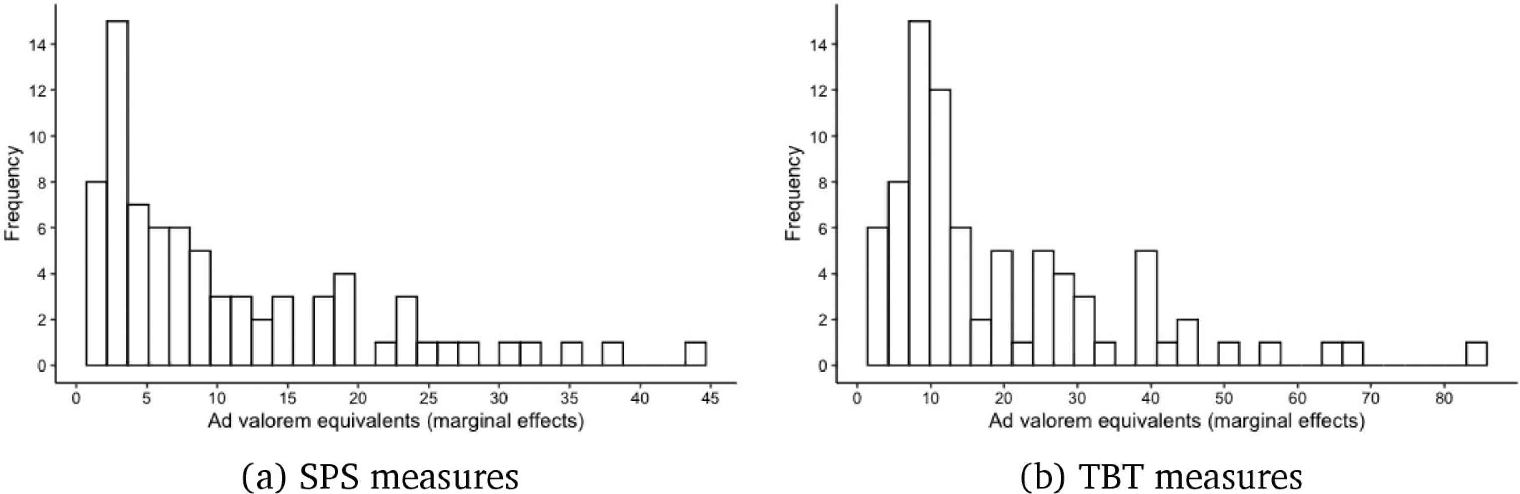
Distribution of AVEs for agricultural products at the country level. Notes: This graph shows the distribution of statistically significant AVEs for all country pairs and products (HS01–HS24). For SPS and TBT measures, we obtained 82 and 89 statistically significant AVEs, respectively. Here, we only keep and report coefficient estimates that are positive since we do not expect standards to induce price reductions.
We estimate the quantity regressions to assess the potential market creation effects of NTMs. Contrary to the price regressions, negative estimates in the quantity regression are not aberrations. NTMs are expected to restrict trade because of the associated trade costs (see, e.g., Fiankor et al., 2021a, 2021b). Positive estimates would imply that country pairs trade more in the presence of standards. This is also not an aberration. Indeed, if the price-signalling effect of a given NTM is strong enough, it may increase import demand of the affected product, despite its cost-raising effect. Null effects from the quantity regressions also offer important information; combined with a positive AVE from the corresponding price regression, they indicate that the price-raising effect of a given NTM and its market-creating effect compensate for each other, resulting in no changes in trade flows for the affected product. Figure 3 shows the distribution of the quantity estimates for the whole sample, i.e., all country pairs and products (HS01–24).15 The general observation is that standard-like NTMs have both trade- enhancing and trade-impeding effects.
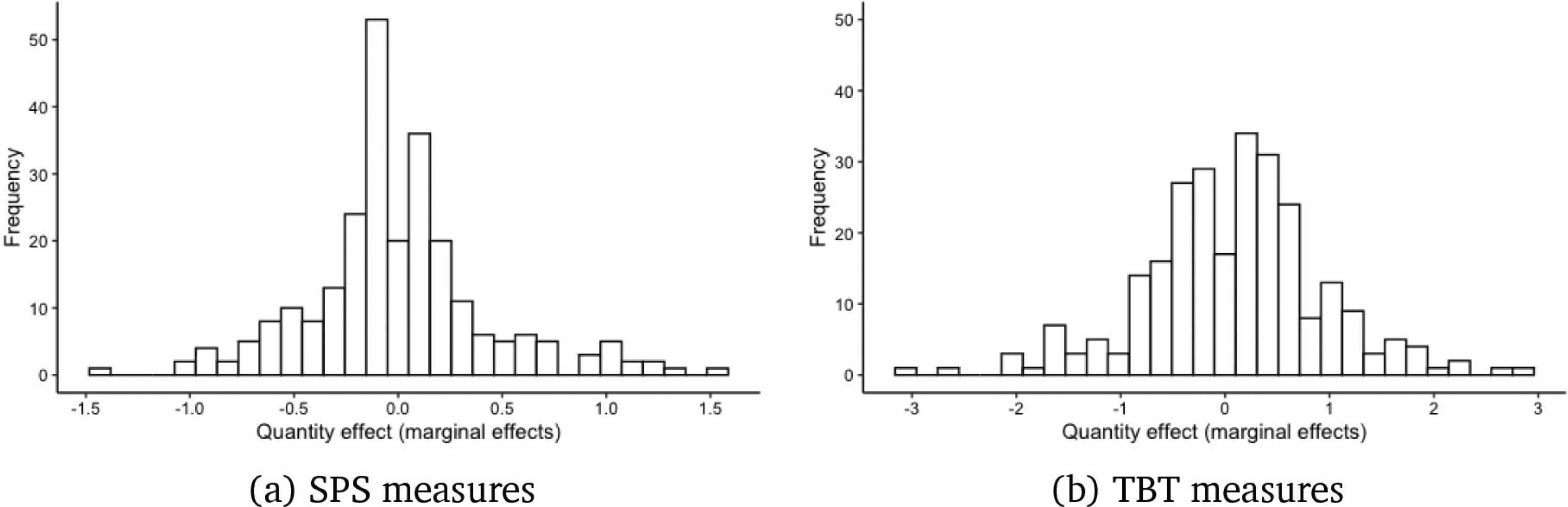
Distribution of changes in trade volume at the country–product level. Notes: This graph shows the distribution of statistically significant quantity estimates for all country pairs and products (HS01–HS24). For the SPS and TBT measures, we obtained 272 and 273 statistically significant trade-volume effects, respectively. The general observation is that standards have both trade-enhancing (positive marginal effects) and trade-impeding (negative marginal effects) effects.
Combining the AVE and quantity estimates, we depict graphically the average equilibrium changes resulting from the imposition of SPS and TBT measures across country pairs and products over time (Figure 4). We observe similar patterns in both figures. A number of AVEs lie in the positive area of the quantity distribution. This means that for many products in the dataset, the demand-enhancing effect of standards can indeed be substantial enough to increase the volume of trade despite the price-raising effect. These results are more pronounced for TBTs. Yet, because the majority of quantity–AVE estimate combinations lie on the vertical zero line, it implies that for most agrifood products, quantity demanded remains unchanged despite higher prices.
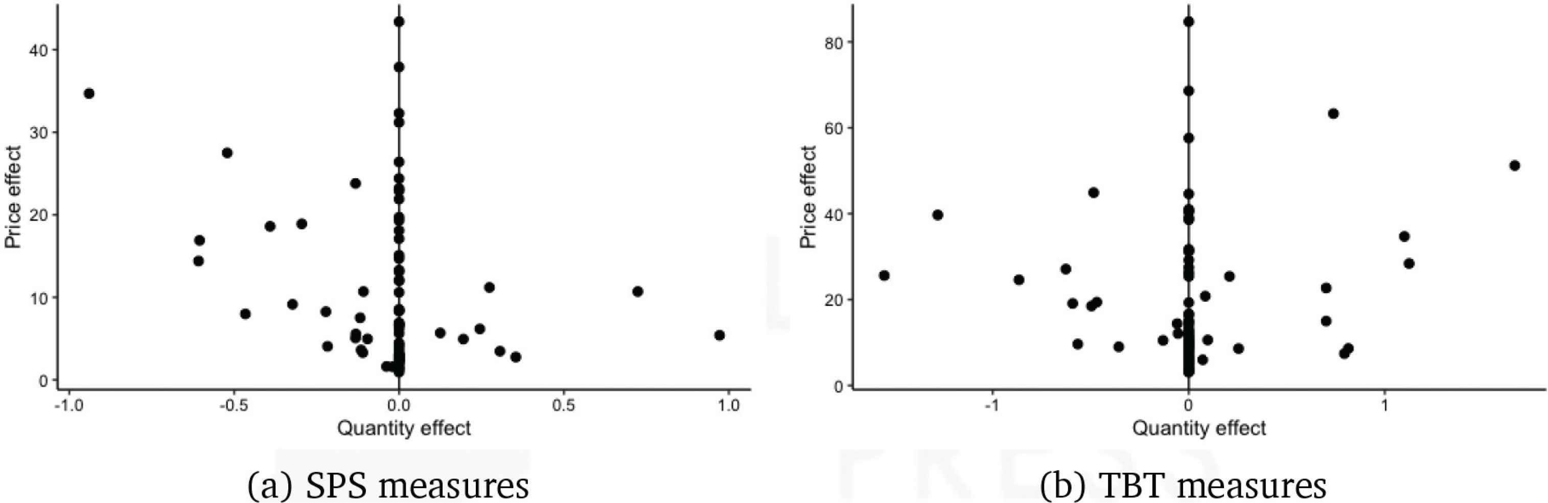
Equilibrium changes in trade volume and prices for agricultural products. Notes: Panels (a) and (b) show combinations of price and quantity estimates obtained from regressions with country-pair FE and year fixed effects (Equation 4). Here we focus on products for which our SPS and TBT measures have a cost- raising effect, i.e., products for which price regressions produced a positive and statistically significant SPS and TBT effect. For example, if the estimated SPS coefficient for product 101105 in the price equation is either statistically insignificant or negative, then the product is not reported in the equilibrium graph. However, if the estimated coefficient is positive and statistically significant, then the AVE is reported on the y-axis and matched with its corresponding quantity estimate on the x-axis. For SPS and TBT measures, we have 81 and 87 positive and statistically significant unit value estimates, respectively.
4.2. Fruit, Nut, and Vegetable Trade Between SSA and High-income OECD Countries
In the previous section, we confirmed that across all countries and products, standards increase product prices, but can have positive, negative, and null trade effects. In this section, we use the so-called “route approach” to isolate these effects specifically for edible fruits, vegetables, and nuts exported from SSA to high-income OECD countries. The estimation strategy corresponds to Equations (2) and (3). The results are presented in Table 2. The variables of interest are SPSsijt−1 × SSAi × OECDj and TBTsijt−1 × SSAi × OECDj, i.e., SPS/TBT applied by high-income OECD countries on imports from SSA, lagged by one period. Using factor notation, the coefficient on the NTM variables and the different regions is directly the marginal effect for that particular region and not the additional effect of the particular route.
| ln Unit valuesijt | Quantitysijt | |
|---|---|---|
| (1) | (2) | |
| SPSsijt−1 × SSAi × OECDj | 0.005*(0.003) | 0.080** (0.036) |
| TBTsijt−1 × SSAi × OECDj | 0.010 (0.009) | 0.031 (0.090) |
| OtherNTMsijt−1 | 0.021*** (0.004) | 0.013 (0.053) |
| ln (1 + Tariffsijt−1) | 0.005 (0.004) | 0.047 (0.050) |
| PTAijt | 0.114*** (0.016) | 0.287** (0.128) |
| WTOijt | 0.0184 (0.074) | 0.346 (0.332) |
| ln Distanceij | 0.173*** (0.010) | 0.845*** (0.066) |
| Contiguityij | 0.036 (0.022) | 0.434*** (0.146) |
| Common languageij | 0.012 (0.013) | 0.276* (0.145) |
| Importer-year fixed effects | Yes | Yes |
| Exporter-year fixed effects | Yes | Yes |
| Product-year fixed effects | Yes | Yes |
| Observations | 290,669 | 290,669 |
Notes: Robust country-pair-product clustered standard errors in parentheses.
***, **, and *denote significance at 1%, 5%, and 10%, respectively. Intercepts included but not reported. Column (1) is estimated using OLS and column (2) is estimated using PPML.
The effect of NTMs on exports of vegetables, fruits, and nuts from SSA to high-income OECD countries
Estimates of the first triple interaction term show that SPS measures have a positive and statistically significant effect on both the price and quantity of vegetables, fruits, and nuts exported from SSA to the OECD. The marginal AVE of one additional SPS measure is 0.5%.16 This effect is comparable in magnitude to those obtained by Sanjuán et al. (2019) for cattle meat (0.8%), white meat (0.5%), and dairy (0.2%). On the trade-volume effects of SPS measures, our results suggest a positive and statistically significant effect. This implies that in our particular setting, their signalling effects surpass their compliance cost effect. This confirms the findings in Kareem and Rau (2018) for African exports of fruits, especially bananas, to the EU. However, compared to Kareem and Rau (2018), our effect sizes are smaller.17 For TBT measures, we observe no price or quantity effects. Combining trade volume and price effects, we can conclude that, despite their price-raising effect, compliance with SPS measures has a demand-enhancing effect.
Note, however, that these positive trade effects are at the intensive margin, i.e., conditional on market entry, confirming earlier findings by Xiong and Beghin (2014) and Crivelli and Gröschl (2016). This indicates that standards impose high fixed and variable costs of trading. Exporters that can enter the market despite the existence of SPS measures are most probably those that have enough capacity to overcome the entry barrier posed by their imposition. Fruits, nuts, and vegetables, which we study, belong to a group of high-value agrifood products that are very much affected by SPS measures. The expectation here is that exporters that comply with SPS measures and are able to show proof of compliance have a significant advantage over non-compliant exporters and, therefore, may see their exports increase significantly. Thus, for SSA countries, failure to comply with SPS measures will exclude them from high-value OECD agrifood markets. However, successful producers from SSA will sell higher volumes at higher prices.
All other import-related NTMs, i.e., OtherNTMsijt, have a price-increasing effect but do not induce significant increases in trade volume. For bilateral tariffs, we do not find any statistically significant effects on both trade and unit values.18 All other traditional gravity variables, when statistically significant, have the expected signs. The presence of a preferential trade agreement (PTA) decreases unit values by 11.4% and increases traded volume by 28.7 tons.19 Consistent with Baldwin and Harrigan (2011)—and many workhorse trade models—that show that zero exports and export unit values are increasing in distance, we find that price increases by around 2% and trade volumes decrease by around 8% if the distance between two partners increases by 10%.
4.3. Robustness Checks
In this section, we expose our main results to three forms of robustness checks. Our benchmark model estimations use a one-year lag of the NTM variables. As a first check of the robustness of our findings, we use the contemporaneous counts of NTMs. The changes in the economic magnitudes we observe (row 2 in Table 3) are minor, such that lagging the counts of NTMs by one period may not suffice to observe differential effects, as it may take much longer for the real effect of a measure to manifest. The implication here for future research would be to have a longer period of analysis to be able to have NTMs lagged by two to three periods. In the final set of robustness checks, we use two different sets of fixed effects in our baseline model specification. In row 3, we include time-invariant country and product fixed effects and year fixed effects. We do this to bring our results as close as possible to Sanjuán et al. (2019), since this is the first study to use the route approach in combination with count and bilateral NTM variables. Finally, in row 4, we include dyadic fixed effects and year fixed effects to bring our findings close to the product-specific estimations in Equation (4). In all cases, our main results remain qualitatively the same with only minor changes in the economic magnitudes. The similarity of the results with the three different sets of fixed effects is reassuring and provides evidence that our main conclusions are invariant to a particular model specification.
| SPSsijt−1 × SSAi × OECDj | TBTsijt−1 × SSAi × OECDj | |||
|---|---|---|---|---|
| ln Unit valuesijt | Quantitysijt | ln Unit valuesijt | Quantitysijt | |
| (1) | (2) | (3) | (4) | |
| (1) Benchmark specifications | 0.005* | 0.080** | 0.010 | −0.031 |
| (2) Contemporaneous NTM | 0.005* | 0.080** | 0.010 | −0.029 |
| (3) Fixed effects (fes, fei, fej, fet) | 0.007** | 0.085** | 0.005 | −0.012 |
| (4) Fixed effects (feij, fet) | 0.008** | 0.092* | −0.036*** | 0.001 |
Notes: Robust country-pair-product clustered standard errors in parentheses.
***, **, and *denote significance at 1%, 5%, and 10% respectively. Exporter-time, importer-time, and product-time fixed effects are included in all regressions.
Robustness checks
Our main models explore the effects across the aggregate group of fruits, vegetables, and nuts while accounting for product fixed effects. Here, we do a deeper search for patterns, by splitting the sample along the three commodities. The results are presented in Table A2 in the appendix. Our main findings remain largely the same, but there are also notable heterogeneities across products. The price-increasing effects of standards are confirmed across all three products. However, we see a trade enhancing effect for vegetables, a null trade effect for fruits, and a trade-reducing effect for nuts. These findings reflect the state of the empirical literature: the standards–trade effect is largely an empirical question that may vary along different dimensions including products, country income classes, and export shares (Santeramo and Lamonaca, 2019a; Fiankor et al., 2021b).
5. CONCLUSION
As developed countries lower their use of custom tariffs and other traditional trade barriers as tools to regulate trade, we have seen an upsurge in standard-like non-tariff measures. While standards can indeed be barriers to trade by imposing costs for trade, they can also be instruments for market creation by addressing information asymmetries, mitigating consumption risks, and enhancing sustainability. In this paper, we disentangled the increased trade costs and demand-enhancing effects of sanitary and phytosanitary (SPS) and TBT measures imposed on fruit, nut, and vegetable trade between sub-Saharan African countries and high-income OECD member states. We found that non-tariff measures (NTMs) increase trade costs and unambiguously raise unit values—either through passed-on compliance costs, quality upgrading, or a combination of the two mechanisms—but they also increase trade volume. For technical barriers to trade (TBT) measures, the signalling effects are not strong enough to induce a demand-enhancing effect. There are also no associated price effects for TBTmeasures.
Overall, we see that compliance with standards bears the potential to improve the integration into the global value chain for exporters of agrifood products fromsub-Saharan Africa (SSA) by guaranteeing them higher sales volumes at higher prices. BecauseMFN tariffs are at alltime lows in many developed countries, the potential gains fromtrade for the least developed countries stemfromreductions in NTMsmore broadly, but standard-like NTMs in particular. Nevertheless, the complexity of NTMs means that this is not an easy task. Trade facilitation measures in the domain ofNTMs and more engagement by governments of the concerned countries would enhance the conditions necessary for SSA countries to better use NTMs to achieve their development goals. Standards harmonisation,mutual recognition, and benchmarking local standards in SSA to international standards are also potential cost-minimising mechanisms that will enhance compliance with standards.
Our study is not without limitations. Heterogeneous effects across countries cannot be estimated within our model specification. Yet, the trade effects and especially the cost effects are expected to vary across countries (Xiong and Beghin, 2014; Rial, 2014) or to depend on market shares (Fiankor et al., 2021b). It may also be misleading to consider ad valorem equivalent (AVE) measures of NTMs as a pure trade-cost effect. The change in market structure—e.g., small firms exiting the market because they cannot comply with NTMs—induced by standards confers more market viability to surviving firms (Asprilla et al., 2019) who may then charge higher prices (Fiankor et al., 2021a). Thus, the increase in trade unit values captures the effect of NTM compliance costs, but may also be a market expansion effect (Cadot et al., 2018b). Our estimates capture the effects of NTMs on existing trade relationships, but not the extensive trade margins, which may also be important in understanding the full effect of NTMs. There is some evidence that SPS measures are more stringent at the extensive margin of trade than at the intensive margin (Ferro et al., 2015; Crivelli and Gröschl, 2016).
CONFLICTS OF INTEREST
The authors declare they have no conflicts of interest.
AUTHORS’ CONTRIBUTION
ADT and DDDF worked together on this paper at all stages: conceptualization the idea, data curation, formal analysis and writing and revising different versions of the paper.
FUNDING
This research was financially supported by the long-term EU-Africa research and innovation partnership on food and nutrition security and sustainable Agriculture LEAP-Agri (Project ‘Agricultural Trade and Market Access for Food Security: Micro- and Macrolevel Insights for Africa’). The project was also supported by funds of the Federal Ministry of Food and Agriculture (BMEL) based on a decision of the Parliament of the Federal Republic of Germany via the Federal Office for Agriculture and Food (BLE). The authors are grateful to the editor and anonymous referees for their constructive comments. The views and opinions expressed in this paper are those of the authors and do not necessarily reflect the official policy or position of the GIZ.
APPENDIX
A.1. Conceptual Framework
To disentangle the effects of NTMs into trade-cost and demand-enhancing effects, we follow closely the conceptual frameworks of Xiong and Beghin (2014) and Cadot et al. (2018b). Assuming constant elasticity of substitution (CES) of demand for agricultural goods produced domestically and those produced abroad, it follows that a given consumer C in importing country j maximises consumption utility subject to a budget constraint
The dual effect of NTMs on the value of import demand can already be identified from Equation (2). The NTM determines
The second step is to derive the export supply. Let us assume that a given producer M for sector s20 in origin country i has a production capacity of Qsi, a technology characterised by a constant elasticity of transformation (CET), which allows M to export to different destinations. The challenge here for producer M is deciding which market to export to and how much to supply. This maximisation problem is expressed by Xiong and Beghin (2014) as follows:
Equating Equations (2) and (5) under the market clearing condition, the equilibrium price in sector s for trade between i and j gives
Cadot et al. (2018b) combine Equations (11) and (12) to solve for the equilibrium quantity in sector s for trade between i and j, yielding our final estimation equation:
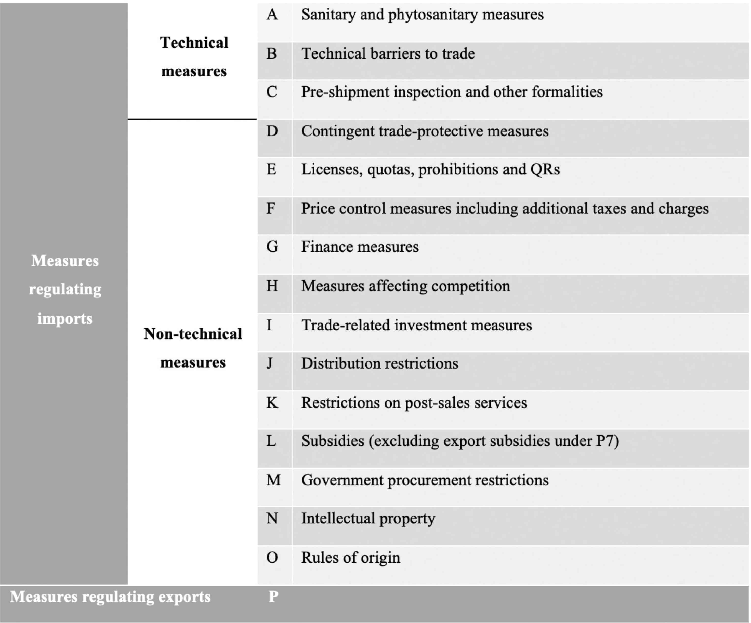
Chapter organisation of NTM in the MAST. Source: UNCTAD and World Bank (2018).
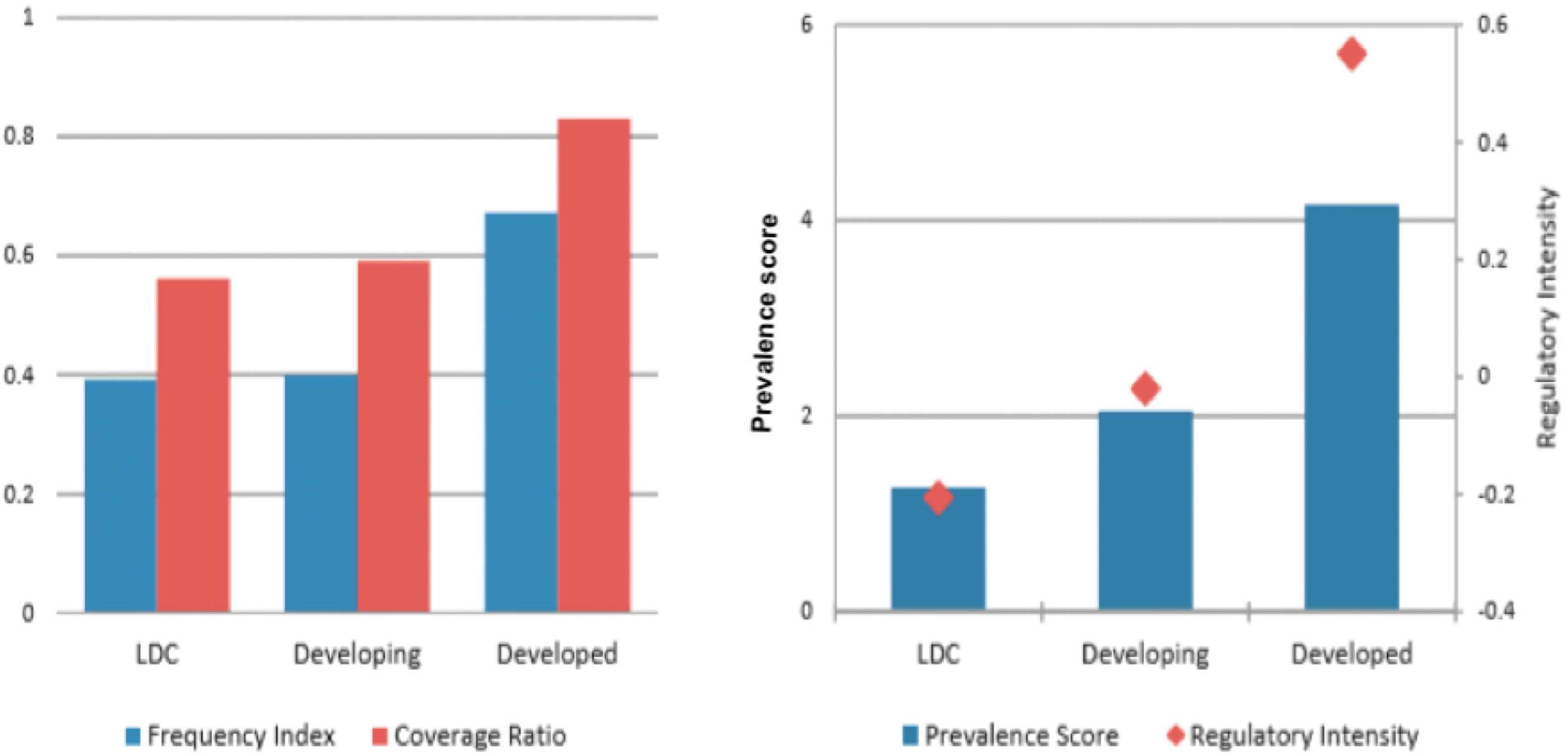
Use of NTMs on imports by income level. Source: UNCTAD and World Bank (2018).
| OECD |
| Australia, Austria, Belgium, Canada, Denmark, Estonia, Finland, France, Germany, Greece, Iceland, Ireland, Israel, Italy, Japan, South Korea, Netherlands, New Zealand, Norway, Portugal, Spain, Sweden, Switzerland, United Kingdom, United States of America |
| SSA |
| Angola, Benin, Burkina Faso, Burundi, Cameroon, Cape Verde, Central African Republic, Chad, Comoros, Democratic Republic of the Congo, Republic of the Congo, Cote d’Ivoire, Equatorial Guinea, Eritrea, Ethiopia (excludes Eritrea), Gabon, The Gambia, Ghana, Guinea, Guinea-Bissau, Kenya, Liberia, Madagascar, Malawi, Mali, Mauritania, Mauritius, Mozambique, Niger, Nigeria, Rwanda, Sao Tome and Principe, Senegal, Seychelles, Sierra Leone, Somalia, South Africa, South Sudan, Sudan, Tanzania, Togo, Uganda, Zambia, Zimbabwe |
| Full sample (excluding OECD and SSA) |
| Afghanistan, Albania, Algeria, American Samoa, Andorra, Anguilla, Antigua and Barbuda, Argentina, Armenia, Aruba, Azerbaijan, The Bahamas, Bahrain, Bangladesh, Barbados, Belarus, Belize, Bermuda, Bhutan, Bolivia, Bonaire, Bosnia and Herzegovina, Brazil, British Indian Ocean Ter., British Virgin Islands, Brunei, Bulgaria, Cambodia, Cayman Islands, Chile, China, Christmas Island, Cocos (Keeling) Islands, Colombia, Comoros, Cook Islands, Costa Rica, Croatia, Cuba, Curacao, Cyprus, Czech Republic, Dominica, Dominican Republic, East Timor, Ecuador, Egypt Arab Rep., El Salvador, Estonia, Falkland Islands, Fiji, French Polynesia, French Southern Territories, Georgia, Gibraltar, Greenland, Grenada, Guam, Guatemala, Guyana, Haiti, Honduras, Hong Kong, Hungary, India, Indonesia, Iran, Iraq, Jamaica, Jordan, Kazakhstan, Kiribati, North Korea, Kuwait, Kyrgyzstan, Laos, Latvia, Lebanon, Libya, Lithuania, Macao, Macedonia, Malaysia, Maldives, Malta, Marshall Islands, Mexico Micronesia, Moldova, Mongolia, Montenegro, Montserrat, Morocco, Myanmar, Nauru, Nepal, New Caledonia, Nicaragua, Niue, Norfolk Island, Northern Marianas, Oman, Pakistan, Palau, Palestine, Panama, Papua New Guinea, Paraguay, Peru, Philippines, Pitcairn, Poland, Portugal, Qatar, Romania, Russia, Saint Barthelemy Saint Helena, Saint Kitts and Nevis, Saint Lucia, Saint Pierre and Miquelon, Saint Vincent and the Grenadines, Samoa, San Marino, Sao Tome and Principe, Saudi Arabia, Senegal, Serbia, Seychelles, Sierra Leone, Singapore, Saint Maarten, Slovakia, Slovenia, Solomon Islands, Somalia, Sri Lanka, Suriname, Syria, Taiwan, Tajikistan, Thailand, Tokelau, Tonga, Trinidad and Tobago, Tunisia, Turkey, Turkmenistan, Turks and Caicos Islands, Tuvalu, Ukraine, United Arab Emirates, Uruguay, Uzbekistan, Vanuatu, Venezuela, Viet Nam, Wallis and Futuna Islands, Yemen |
List of importing and exporting countries
| Vegetables | Fruits | Nuts | ||||
|---|---|---|---|---|---|---|
| ln UVsijt | Qsijt | ln UVsijt | Qsijt | ln UVsijt | Qsijt | |
| (1) | (2) | (3) | (4) | (5) | (6) | |
| SPSsijt−1 × SSAi × OECDj | 0.007**(0.004) | 0.029*(0.015) | 0.008**(0.003) | −0.001 (0.044) | 0.015 (0.009) | −0.245*** (0.087) |
| TBTsijt−1 × SSAi × OECDj | 0.027***(0.010) | −0.042 (0.068) | −0.020**(0.009) | −0.073 (0.106) | 0.002 (0.030) | 0.009 (0.264) |
| OtherNTMsijt−1 | 0.016***(0.006) | 0.206***(0.069) | 0.033***(0.005) | 0.013 (0.044) | −0.009 (0.013) | 0.251** (0.111) |
| ln (1 + Tariffsijt−1) | −0.008*(0.004) | 0.036 (0.047) | −0.015***(0.004) | −0.006 (0.036) | −0.020**(0.009) | −0.013 (0.067) |
| PTAijt | −0.115***(0.019) | 0.164 (0.157) | −0.093***(0.017) | 0.484***(0.134) | −0.136***(0.021) | 0.068 (0.221) |
| WTOijt | −0.041 (0.083) | 0.183 (0.364) | −0.048 (0.064) | 0.033 (0.409) | −0.086 (0.116) | 1.840*** (0.688) |
| ln Distanceij | 0.184***(0.011) | −0.947***(0.082) | 0.160***(0.011) | −0.964***(0.072) | 0.059***(0.012) | −0.371** (0.151) |
| Contiguityij | −0.050**(0.023) | 0.375**(0.170) | −0.045*(0.024) | 0.490***(0.138) | −0.023 (0.030) | 0.553** (0.216) |
| Languageij | 0.000 (0.015) | 0.373**(0.168) | −0.025*(0.014) | 0.210*(0.114) | 0.002 (0.018) | −0.059 (0.168) |
| Observations | 170,175 | 170,175 | 148,707 | 148,707 | 39,065 | 39,065 |
Notes: Robust country-pair-product clustered standard errors in parentheses.
***, **, and * denote significance at 1%, 5%, and 10%, respectively. Exporter-time, importer-time, and product-time fixed effects are included in all regressions. Intercepts included but not reported. The models in the even-numbered columns are estimated using OLS while those in the odd-numbered columns are estimated using PPML. The products are classified as follows: Vegetables HS 07 (070110–071490), Fruits HS 08 (080310–081400), and Nuts HS08 (080111–08290). The corresponding HS-codes for this classification are from the TradeMap, which is not a perfect match with the GTAP classification (product code 4 – vegetables, fruit, nuts) used in our main model for exploring the effect across all three product groups.
Effect of NTMs on exports from SSA to high-income OECD countries; by product categories
Footnotes
For example, labelling requirements alleviate asymmetric information, maximum residue limits mitigate health risks, and quarantines protect the environment from the spread of pests and diseases.
While the standards–trade effect may look similar to tariffs (e.g., raising import prices), strict comparisons between the two are not valid. In a small, open economy, the socially optimal tariff level is zero. This is not necessarily the case for standards. A call for zero standards ignores their potential benefits to the consumer, producer, and society. At home, the optimal standard must consider the marginal gain in utility for consumers and the marginal cost for producers. Tariffs are by construction trade-reducing, but standards may also be market-creating measures. For a detailed theoretical discussion on the economics of NTMs, we refer the reader to de Melo and Shepherd (2018).
See Santeramo and Lamonaca (2019a) for a review.
The ad valorem equivalent is the level of ad valorem duty that would have the same trade effect as the NTMs under consideration. This allows for a direct comparison with ad valorem tariffs and thus for a quantitative estimation of the impact of NTMs on economic outcomes such as trade flows (Looi Kee et al., 2009). Alternatively, Cadot et al. (2018b) define them as a proportional increase in the import price of a good to which a given NTM is applied relative to a counterfactual where it is not applied.
For a detailed review, see Santeramo and Lamonaca (2019b).
Xiong and Beghin (2014) measured NTMs as maximum residue limits. In so doing, they provide precise estimates on the effects of a specific standard on trade flows but lose the generality of studies using counts of SPS notifications, which cover a broad range of policy instruments. However, since many notifications in these databases also relate to MRLs, we think our contribution is valuable.
Alternatively, we could use a dummy variable to account for the presence or otherwise of an NTM. However, with time it is hard to find sectors and country pairs where no NTMs are applied. Using a dummy in such situations will make it difficult to isolate the desired economic effect. Moreover, the use of dummies is problematic because we then implicitly assume that the effect of one NTM is not different from the effect of several NTMs. It is more intuitive to believe th7at the compliance cost increases with the number of NTMs (cumulative burden). Nevertheless, in a recent study on the dual trade effects of SPS and TBT measures on Chinese pork imports, Peci and Sanjuán (2020) arrive at similar conclusions when using the count measure and the simple dummy. A similar conclusion is reached in Fiankor et al. (2021b) for specific trade concerns raised on SPS measures.
An alternative to the “interaction or route approach” is to limit the sample to only SSA exporters and OECD importers.
Ideally, domestic prices should be used to measure Psijt. However, such prices are not comparable across countries, which is a condition necessary for our analysis. Instead, as a proxy, we use unit values. Unit values are, however, not perfect proxies since they are border prices (cost, insurance, and freight), which are usually not what the final consumer pays for the product. This is not an issue in our work, however, since the SPS and TBT measures we focus on are both price-increasing measures as a result of the compliance costs associated with them. The issue that trade unit values do not reflect the final price consumers pay is more of a concern for non-technical measures, where CIF prices will likely not reflect shadow prices. This production cost increase is expected to be passed through to CIF prices, with the degree of pass-through depending on the market structure (Cadot et al., 2015). Data on unit values can also be very noisy, e.g., due to reporting mistakes by customs officers. This does not threaten our identification strategy, as long as these measurement errors are not systematic in the dataset (Cadot et al., 2018a).
de Melo and Nicita (2018) highlight several limitations in the NTM dataset provided by TRAINS. Little or no information is provided on the actual stringency of each measure. Interpreting higher counts of NTMs on a particular good as higher stringency is not straightforward, since one measure can be more stringent than several measures combined. The assumption that a cumulative burden is equivalent to higher compliance costs may not always be true. Also, some measures are related to each other, implying a risk of collinearity when trying to estimate the effects of many individual measures. However, by aggregating NTMs into chapters (SPS and TBT) we attempt to reduce the significance of this issue. Another limitation relates to the time dimension of the data. Data that existed for a long time and never changed are not accounted for in the data. Also of concern is the starting date recorded in the database being interpreted as the beginning of the implementation of a specific measure. New measures may replace similar measures that were not in the database before. Yet, because our study focuses on a recent analysis period (2012–2016) we mitigate this concern.
Another approach to capture product-specific effects is to have the interact the SPS and TBT variables interact with each product. However, this will result in too many estimates in one equation (899 products at the HS 6-digit level in the dataset). We run the risk of running out of degrees of freedom. Instead, we run the regression models separately for each HS6 digit product in HS01–HS24.
At the product level, there is low variation in the number of bilateral NTMs across countries, as most of them are applied uniformly by each importer on products from all origins (i.e., in most cases, NTMsijt = NTMsjt). By including importer-time fixed effects at the product level, we run the risk that all our NTM estimates are captured by the importer-time fixed effects. For this reason, we include bilateral fixed effects for country-pair varying effects and year fixed effects to account for possible economic shocks over the period from 2012–2016.
With average and median R2 values of 0.83, the overall fit of the unit value equations is very good across the different products.
To ensure that we are able to showa clean distribution of the AVEs, we drop outliers. Following Ghodsi et al. (2016), we define outliers as AVEs that are above the maximum value across country–product pairs, where the maximum value is calculated by multiplying the interquartile range (IQR = Q3 − Q1) by 3 and adding it to the value for the third quartile (Q3) of the distribution. Thus, outliers are all those estimates that lie above the value Q3 + (3 × IQR).
Since both positive and negative estimates are kept for the quantity regression, an interval is defined following Ghodsi et al. (2016), and estimates lying out of this interval are considered outliers that are consequently dropped to improve visualisation. The maximum value for the interval is calculated the same way as it was done for the price regression, i.e., Q3 + (3 × IQR). The minimum value is calculated by multiplying the interquartile range (IQR) by 3 and subtracting it from the value of the first quartile (Q1) of the distribution [Min Value = Q1 − (3 × IQR)]. Thus, the interval for quantity estimates reported here is [Q1 − (3 × IQR); Q3 + (3 × IQR)].
The assumption here is that an increase in the number of SPS measures from 2 to 3 is the same as from 30 to 31. This is a rather strong assumption that we acknowledge as a limitation of our present work. For example, if a product had two NTMs imposed on it, then the marginal effect of increasing the number of NTMs on this particular product by one more unit is expected to be higher compared to a product where 30 NTMs are already applied.
The model specifications in Kareem and Rau (2018) do not account for time-varying country fixed effects—which they instead capture using country GDPs and institutional quality in their models. By including country-time fixed effects in our models, we capture much of the country-specific time variations that may also be driving bilateral trade, explaining our substantially smaller effect.
An interesting exercise would have been to be able to directly compare the AVE of NTMs with the tariff effect. Cadot et al. (2018b) estimates the AVE of NTMs in agrifood products to be around three times larger on average than for tariffs. However, many SSA countries are beneficiaries of preferential trade regimes from many of the OECD member states (e.g., GSP, EPA, EBA, and AGOA), and this may explain the insignificant negative effects for tariffs.
The price effect we observe for PTAs may appear to contradict the literature on quality upgrading as a response to a tariff liberalisation scenario where we expect a positive effect on unit values. Nevertheless, because multilateral trade agreements lower trade barriers on imported goods, which might affect export prices not only through a cost effect but also through access to better quality products, their net effect on export prices is a priori unclear (Flach and Gräf, 2020).
“s” is used interchangeably for good (consumer side) and sector (producer side).
REFERENCES
Cite this article
TY  - JOUR
AU  - Aristide Djimgou Tchakounte
AU  - Dela-Dem Doe Fiankor
PY  - 2021
DA  - 2021/09/21
TI  - Trade Costs and Demand-Enhancing Effects of Agrifood Standards: Consequences for Sub-Saharan Africa
JO  - Journal of African Trade
SP  - 51
EP  - 64
VL  - 8
IS  - 1
SN  - 2214-8523
UR  - https://doi.org/10.2991/jat.k.210907.001
DO  - 10.2991/jat.k.210907.001
ID  - Tchakounte2021
ER  -