
Bayesian lead time estimation for the Johns Hopkins Lung Project data
Tel.: +1 502 852 8078.
Tel.: +1 502 852 3525.
- DOI
- 10.1016/j.jegh.2013.05.001How to use a DOI?
- Keywords
- Lead time; Lifetime distribution; X-ray screening; Lung cancer
- Abstract
Problem statement: Lung cancer screening using X-rays has been controversial for many years. A major concern is whether lung cancer screening really brings any survival benefits, which depends on effective treatment after early detection. The problem was analyzed from a different point of view and estimates were presented of the projected lead time for participants in a lung cancer screening program using the Johns Hopkins Lung Project (JHLP) data.
Method: The newly developed method of lead time estimation was applied where the lifetime T was treated as a random variable rather than a fixed value, resulting in the number of future screenings for a given individual is a random variable. Using the actuarial life table available from the United States Social Security Administration, the lifetime distribution was first obtained, then the lead time distribution was projected using the JHLP data.
Results: The data analysis with the JHLP data shows that, for a male heavy smoker with initial screening ages at 50, 60, and 70, the probability of no-early-detection with semiannual screens will be 32.16%, 32.45%, and 33.17%, respectively; while the mean lead time is 1.36, 1.33 and 1.23 years. The probability of no-early-detection increases monotonically when the screening interval increases, and it increases slightly as the initial age increases for the same screening interval. The mean lead time and its standard error decrease when the screening interval increases for all age groups, and both decrease when initial age increases with the same screening interval.
Conclusion: The overall mean lead time estimated with a random lifetime T is slightly less than that with a fixed value of T. This result is hoped to be of benefit to improve current screening programs.
- Copyright
- © 2013 Ministry of Health, Saudi Arabia. Published by Elsevier Ltd.
- Open Access
- Open access under CC BY-NC-ND license. http://creativecommons.org/licenses/by-nc-nd/4.0/
1. Introduction
Lung cancer, the leading cause of cancer death for both men and women, occurs in the lungs and most often begins in the cells that line the bronchi. Two major types of lung cancer have been identified: small cell lung cancer, which accounts for about 20% of all cases, and non-small cell lung cancer, the most common type. Different types of lung cancers require different kinds of treatments. The age-specific lung cancer incidence rate rises with advancing age and reaches its peak between 65 and 74 [1].
Cancer screening is carried out to detect malignant tumors early, in order to translate into early treatment and a better prognosis. However, there are controversies concerning lung cancer screening since the early 1970s. The benefit of screening is often measured by collecting information on how long patients are alive after the diagnosis, called survival time. The survival time is the time difference between the date the disease is diagnosed and the date a patient dies due to the disease. However, a patient’s survival time is often perceived longer due to the earlier date of diagnosis, even though early detection may not be translated into effective treatment in those days. For example, suppose a screening exam leads to a cancer diagnosis at time t before any symptoms appear, as shown in Fig. 1, then the survival time will be calculated as (td − t), although in fact the survival time is (td − t2). This bias occurs due to the contribution of (t2 − t), which is called the lead time. The lead time is the difference between the time of diagnosis via a screening exam and the time of clinical disease onset without screening [2]. Since the survival benefit of screening heavily relies on the lead time, it is critical to accurately evaluate the distribution of the lead time.
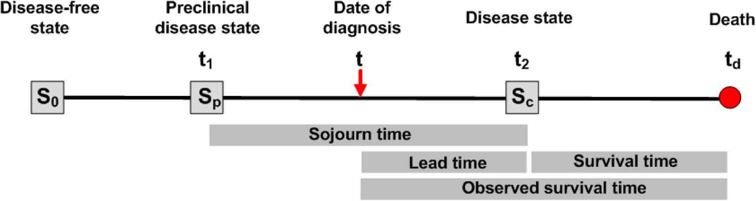
A graphical representation of the disease progressive model.
For this study, the commonly followed disease progressive model is assumed where the disease develops by progressing through three states, denoted by S0 → Sp → Sc [3]. Its graphical representation is illustrated in Fig. 1. The state S0 refers to the disease-free state, where either a person does not have the disease, or the disease is in such an early stage that it cannot be detected by a screening exam. The preclinical disease state, Sp, is a state in which an asymptomatic individual unknowingly has the disease that a screening exam can detect. The disease state, Sc, is a state at which the disease manifests itself with clinical symptoms. If a person enters the preclinical state (Sp) at age t1 and becomes clinically incident (Sc) later at age t2(>t1), then (t2 − t1) is the sojourn time in the preclinical state. However, if this person undergoes a screening exam at time t within the time interval (t1, t2) and cancer is diagnosed, then the length of time (t2 − t) is the person’s lead time.
Many researchers have proposed methods for inference on the lead time among participants in a screening program [4–12], usually by providing formulas to estimate the mean and the variance of the lead time. Wu et al. [2] derived the probability distribution of the lead time for the whole diseased cohort, including both screen-detected cases and interval-incident cases, where the human lifetime was treated as a fixed value. The model allows estimation of the proportion of patients whose lead time is zero and the proportion whose lead time is positive from the program. Later, Wu et al. applied this approach to the Mayo Lung Project (MLP) data to estimate the lead time distribution [13]. However, it is not realistic to fix a person’s lifetime T in the estimation of the lead time distribution. For this reason, [18] developed a model to treat the lifetime T as a random variable and made the estimation of lead time distribution more practical [1]. The main objective of the present study is to evaluate the lead time distribution in lung cancer screening using the Johns Hopkins Lung Project (JHLP) data and the newly developed method with a changing lifetime T.
2. Materials and methods
The design of the JHLP can be found in the literature [14]. The JHLP trials enrolled 10,386 men in the Baltimore metropolitan area between 1973 and 1978, aged 45 years and older at enrollment, who smoked at least one pack of cigarettes per day (or who had smoked this much within 1 year of enrollment) and who had no prior history of respiratory cancer. Then all participants were randomized into two groups: chest X-ray only, or a dual screen (chest X-ray and sputum cytology) group, resulting in 5160 men in the chest X-ray only group and 5226 in the dual-screen group. Participants in the chest X-ray group received a chest X-ray screening test annually for eight consecutive years. If any of the tests was positive, then the screen was considered positive and a definitive work-up exam, such as biopsy, was done. The data that were used in this study were the chest X-ray group, and the data included the number of participants in each screening exam, the number of detected and confirmed cancer cases in each screening exam, and the number of interval cases. These data were stratified by age at study entry from 45 to 88 years old. However, after carefully examining the data, only the data from age 45 to age 70 were used, excluding age groups 47, 58, 62, 68, 69 and ages above 70, because these age groups had very few participants and might cause a large bias in the estimation.
Consider a cohort of initially asymptomatic individuals in a screening program. Let β(t) be the sensitivity of the screening modality, where t is the individual’s age at the exam. Define w(t)dt as the probability of a transition from S0 to Sp during (t, t + dt). Let q(x) be the probability density function (pdf) of the sojourn time in Sp, and let
For an initially asymptomatic male heavy smoker of age t0, who has no history of lung cancer, and suppose that he plans to undergo K screening exams at ages t0 < t1 < … < tK−1. The distribution of the lead time will be a point mass at 0, and a positive continuous probability density. The reason is that for the screen-detected cases, the lead time is greater than zero, while for the interval incident cases, the lead time is zero. A brief summary of the derived probability formulae for the lead time with a changing human lifetime T is given in the Appendix A.
The lead time distribution is a function of the screening sensitivity β(t), the transition probability density w(t), the sojourn time distribution q(x), a person’s initial age at screening, and a future screening frequency or screening schedule. The first three parameters were estimated from the JHLP data using the following parametric models:
In this study, the unknown parameters are θ = (β, μ, σ2, κ, ρ). Markov Chain Monte Carlo (MCMC) was used to draw posterior samples with noninformative priors; each simulation was run for 11,000 iterations, with 1000 burn-in steps, and after the burn-in steps, then the posteriors were sampled every 10 steps. The MCMC trace plots and the posterior density plots of θ are plotted using the final 1000 posterior samples for θ, as can be seen in Figs. 2 and 3. All parameters were converged nicely based on Bayesian output analysis. The posterior means of the parameters are
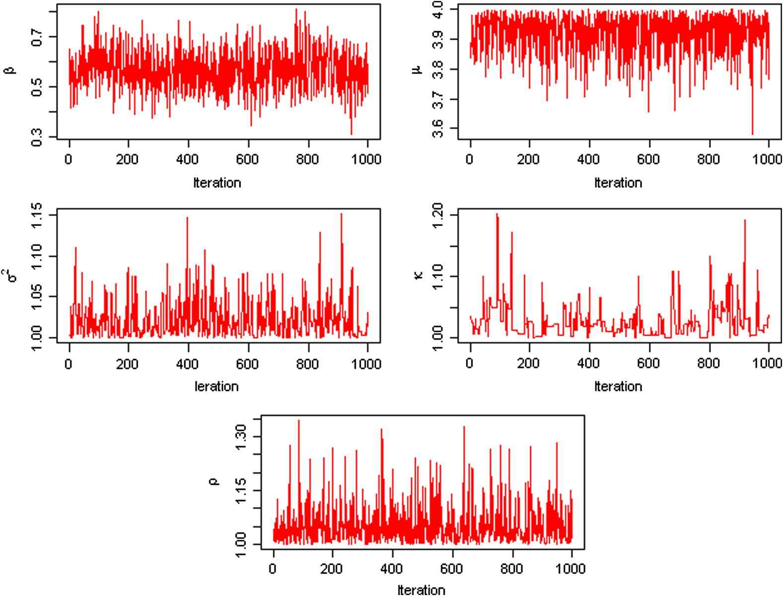
The MCMC trace plots of the parameters θ = (β, μ, σ2, κ, ρ) using the JHLP data.
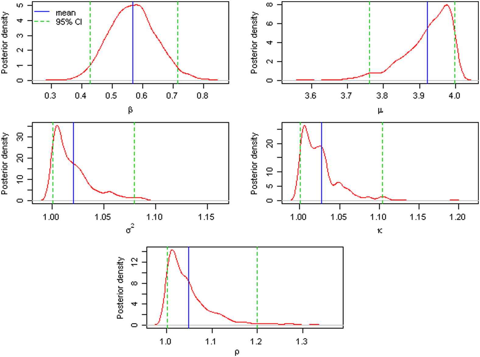
The posterior density plots of the parameters θ = (β, μ, σ2, κ, ρ) using the JHLP data.
| Mean | SDa | 2.5%b | 50%c | 97.5%d | |
|---|---|---|---|---|---|
| β | 0.568 | 0.076 | 0.427 | 0.565 | 0.716 |
| μ | 3.922 | 0.065 | 3.762 | 3.938 | 3.997 |
| σ2 | 1.020 | 0.022 | 1.001 | 1.014 | 1.079 |
| κ | 1.027 | 0.028 | 1.001 | 1.021 | 1.104 |
| ρ | 1.049 | 0.052 | 1.001 | 1.034 | 1.200 |
SD stands for the empirical standard deviation.
The 25th, 50th, and 97.5th percentiles, respectively.
The estimates of the parameters.
3. Results
The Bayesian posterior samples
For simplicity, three cohorts of initially asymptomatic males were chosen, with initial screening age t0 = 50, 60, and 70, respectively. For each cohort, various screening frequencies were examined, with screening interval Δ = 6, 12, 18, and 24 months. The number of screenings K = [(T − t0)/Δ] is a function of the lifetime T, therefore it is a random variable in the simulation. From Eq. (4), the final distribution of the lead time is simply a weighted average of the different lengths of lifetimes.
Table 2 summarizes the Bayesian predictive inference for the lead time. The probability that the lead time is zero and the probability that the lead time is positive are reported as percentages in Table 2. The mean lead time and its empirical standard error were reported in years. The density curves for the lead time are shown in Fig. 4 for different screening intervals when t0 = 60, as the density curves when the initial screening age is 50 or 70 are very similar.
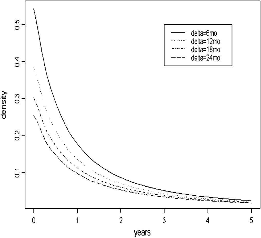
The pdf curve of the lead time when t0 = 60.
| Δa | P0b (%) | 1 − P0 (%) | Mean (yr) | SEc (yr) |
|---|---|---|---|---|
| Age at initial screen t0 = 50 | ||||
| 6 mo | 32.16 | 67.84 | 1.360 | 2.278 |
| 12 mo | 46.30 | 53.70 | 1.168 | 2.224 |
| 18 mo | 54.43 | 45.57 | 1.038 | 2.163 |
| 24 mo | 59.86 | 40.14 | 0.944 | 2.106 |
| Age at initial screen t0 = 60 | ||||
| 6 mo | 32.45 | 67.55 | 1.332 | 2.229 |
| 12 mo | 46.54 | 53.46 | 1.144 | 2.175 |
| 18 mo | 54.58 | 45.42 | 1.018 | 2.116 |
| 24 mo | 59.97 | 40.03 | 0.926 | 2.060 |
| Age at initial screen t0 = 70 | ||||
| 6 mo | 33.17 | 66.83 | 1.230 | 2.077 |
| 12 mo | 47.16 | 52.84 | 1.051 | 2.020 |
| 18 mo | 55.03 | 44.97 | 0.933 | 1.960 |
| 24 mo | 60.22 | 39.78 | 0.848 | 1.905 |
Δ = ti − ti − 1 is the time interval between screens.
P0 = P(L = 0|D = 1) is the probability of “no-early-detection”.
SE stands for the empirical standard error. This is a simulated projection. The number of screens K is a random variable, changing with the lifetime T.
A projection of the lead time distribution using the JHLP control group.
These results suggest that a man who begins semiannual screening (i.e., Δ = 6 months) when he is 60 years old and develops lung cancer sometime during his life has a 32.45% chance that he will not be detected early by the scheduled screening exams. This probability of no-early-detection from the screening program increases to 46.54% if the exams are annual. For a man with initial screening age at 50 [respectively, 70], the probability of no-early-detection with semiannual screens will be 32.16% [or 33.17% for age 70]. The probability of no-early-detection is monotonically increasing when the screening interval increases within the same age group. This probability is slightly increasing as the initial age increases for the same screening interval. The difference between the initial ages 60 and 70 is smaller than that corresponding difference between the initial age groups 50 and 60.
The mean lead time in each age group decreases as the screening time interval increases in Table 2 (i.e., more frequent screening exams will result in longer lead times). The increase in the mean lead time is due partly to the smaller point mass at zero of the lead time when screening intervals are closer together. The standard deviation of the lead time decreases as the time between screening exams increases. The mean lead time and the standard error of the lead time both slightly decrease as age increases within the same screening interval. Table 2 also reveals that the standard deviation for the lead time is greater than the mean lead time.
4. Discussion
The screening sensitivity, the sojourn time distribution, and the transition density were first estimated in a Bayesian framework. The probability distribution of the lead time from the JHLP data was then estimated by employing a newly developed method [1]. This method considers the human lifetime as a random variable using information from the published actuarial life table of the U.S. Social Security Administration to make the screening model more realistic [17].
The sensitivity was considered as a constant parameter across all age groups in this work. Consequently, the estimated sensitivity
The density curves of the lead time of the JHLP study group data (i.e., X-ray and cytology screening) were estimated when the lifetime has a fixed upper bound of 75 years old in the previous study [1]. The density curves with the JHLP control group data (i.e., only X-ray) are more skewed to the right than those of the previous study. This in general suggests that the lead time of the JHLP study group data has a greater effect on early detection owing to additional cytology screening, although the lifetime was treated as a random variable for the JHLP control group data.
Some simulation was done for the new lead time model when lifetime T is a random variable; the purpose is to find which factor will affect the distribution of the lead time more significantly. Screening sensitivity was found to affect the lead time distribution slightly; it plays a bigger role in the proportion of no-early-detection versus the proportion of early-detection. The sojourn time plays the most significant role in the lead time distribution: in general, a longer (shorter) sojourn time will lead to a longer (shorter) lead time. For lung cancer, the distribution of the sojourn time is heavily skewed to the right, with a large variance; that is why the variance of the lead time in lung cancer is also large.
The lead time model used in this study can answer the following two main questions: the probability that a person’s lung cancer will be detected early if a person would develop lung cancer later in life; and the mean/standard error of the lead time for different screening schedules. It is hoped that the results of this study will be beneficial to improving current screening programs.
Conflict of interest
The authors declare that they have no conflict of interest.
Appendix A.
This appendix provides a summary of the key formulae in the lead time distribution [1]. For an initially asymptomatic male with no history of lung cancer who plans to take K screening exams at ages t0 < t1 < … < tK−1. Let D represents the true disease status and L represents the lead time. The lead time distribution given that his lifetime T = tK(>tK−1) is:
References
Cite this article
TY  - JOUR
AU  - Hyejeong Jang
AU  - Seongho Kim
AU  - Dongfeng Wu
PY  - 2013
DA  - 2013/06/14
TI  - Bayesian lead time estimation for the Johns Hopkins Lung Project data
JO  - Journal of Epidemiology and Global Health
SP  - 157
EP  - 163
VL  - 3
IS  - 3
SN  - 2210-6014
UR  - https://doi.org/10.1016/j.jegh.2013.05.001
DO  - 10.1016/j.jegh.2013.05.001
ID  - Jang2013
ER  -