1. COVID-19 PANDEMIC AND MODELS BASED ON PREVIOUS LITERATURE

The COVID-19 pandemic brings a new update to the famous George E. P. Box quote “all models are wrong, but some are useful” [1]. Martin Goodson wrote “All models are wrong, but some are completely wrong” [2]. Many models were produced in a short period by the scientific community and, contrary to what is usual, with vast dissemination to a broad audience by TV, newspapers, and social networks. Unfortunately, bad things seem to outmanoeuvre good ones in spreading speed.

In Portugal, like in other countries, many models appeared in an earlier phase of the pandemic with catastrophic numbers of deaths and infected cases, often without a clear distinction among suspected, symptomatic, asymptomatic, confirmed, and reported cases. Some mathematicians were in the front line, but few statisticians appeared in this phase. Undoubtedly well-intentioned, many non-statisticians and non-mathematicians gave their contributions to help in this hard situation by modelling “something”, but findings were involved in controversy. In fact, without enough and reliable data, it is impossible to establish good models or reliable predictions.

Worldwide, the motto “Let,s flatten the curve” produced a competition between “the best models” to express the number of cases with and without containment measures. In a second phase, a new competition was guessing when would be the peak of the epidemic curve and latter for an end date for this pandemic or the second waves in each country. In Portugal, some serious models were produced, but in newspapers and social networks, some inaccurate references were given to a “normal epidemic curve” and also to a “log-normal curve/distribution”, even using classical sampling statistics to describe properties of the epidemic curve. By then, some statisticians intervened to clarify that there was a confusion between “epidemic curve and probability distribution” and the Portuguese Statistical Society took a position to avoid the dissemination of these wrong concepts. In other countries, we found similar approaches. Rashed et al. [3] studied 16 prefectures in Japan and they stated that the number of daily COVID-19 confirmed cases follow bell-shape or log-normal distribution in most prefectures. At the beginning, some of these curves seemed symmetric, but the bell-shape does not represent a normal distribution or a log-normal distribution.

Looking at different time windows, many curves may emerge, taking different forms over time intervals. Figure 1 expresses the dynamics of new reported cases until the 31 July 2020, according to the European Centre for Disease Prevention and Control, in Portugal and in the Netherlands, Gaussian and lognormal functions were fitted to daily cases from first day to the 10 May 2020 in Portugal and 17 May 2020 in the Netherlands. Dashed lines show discrepancies between predicted and observed daily cases, highlighting how bad these popular models are. Section 3 gives some mathematical details and assumptions about the Gaussian curve.

Figure 1

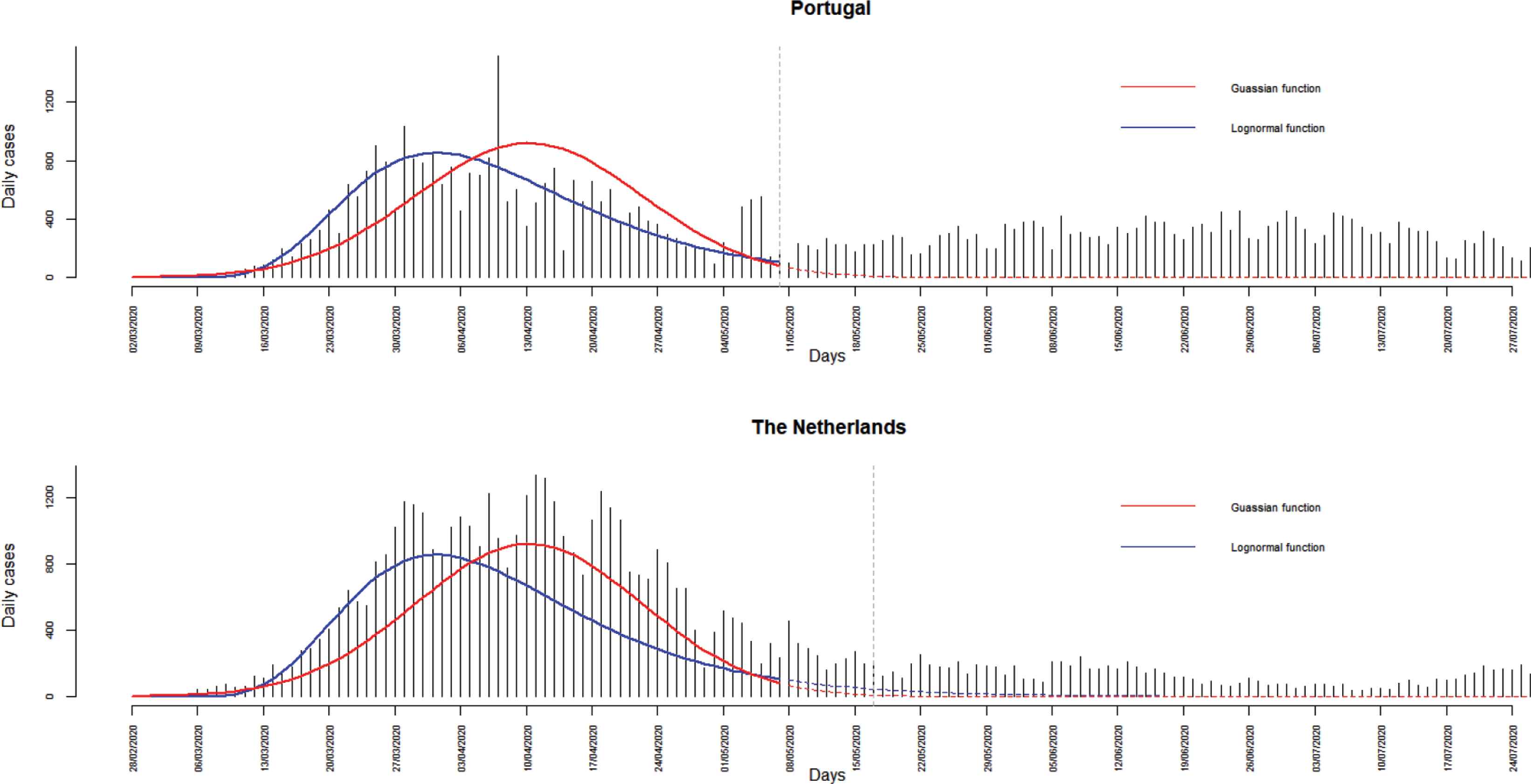
COVID-19 daily cases in Portugal and in the Netherlands until the 31 July 2020. Fitted models (solid lines) and predicted cases (dashed lines) correspond to Gaussian (red) and lognormal (blue) curves. Green vertical lines correspond to the 10 May 2020 in Portugal and to the 17 May 2020 in the Netherlands.

The importance of temporal indexation needs to be present in this type of data and unfortunately this key element has often been ignored. During this debate, advocates of “a normal/log-normal curve” have argued that this is a basic concept explained in first lectures on epidemics and there are many introductory textbooks of epidemiology, describing the epidemic curve as a normal/log-normal distribution. In fact, this confusion appears in several old and recent documents of reputable international institutions, books and important scientific journals [3–8]. For many decades, applied epidemiology training programs of the Centers for Disease Control and Prevention (CDC) have been a crucial impact worldwide and particularly, in African and Asian countries (e.g., Reddy et al. [9]), where outbreaks and epidemics are more frequent. In many low and middle-income countries, teaching materials from several CDC courses are very important references and often unique documents for health professionals. Thus, these crucial documents need to be urgently updated.

2. TIME IS AN IMPORTANT KEY IN EPIDEMIOLOGY AND IN THE EPIDEMIC CURVE

In epidemiology, there are many other curves (e.g., survival curve) and in statistics, there are countless probability distributions (e.g., Weibull, Gamma, and Beta) [10]. These concepts - epidemic curve and probability distribution - are entirely different. In an epidemic situation, we are interested in the epidemic curve that has a particular and fundamental characteristic – cases are indexed by time (e.g., day or week). To visualize an epidemic curve, we put on the vertical axis the number of cases (discrete nature) and the horizontal axis the time unit. The temporal correlation is a key characteristic since new cases are strongly correlated with past cases. The normal distribution is widely used to describe several continuous variables (e.g., body weight). In a probability distribution the values (x) of a random variable (X), are represented on the horizontal axis, and on the vertical axis, it is displayed the density or the probability mass function, according to whether the variable is continuous or discrete. Thus, if we explore the new cases according to a common distribution used to describe the frequency distribution of a random sample, we lose the temporal reference. In fact, the desirable property of independent and identically distributed (i.i.d.) variables, common to most of the biomedical applications, fails in an epidemic curve situation. Moreover, although the epidemic curve may look like a Gaussian curve and be eventually modelled by a Gauss function, it is not a Gaussian (normal) distribution or a log-normal distribution, as some claim [3–7].

3. STATISTICAL RATIONAL

To explain why this confusion may arise, we will consider a toy example with the new cases of an epidemic in T days, denoted by {y_t, t = 1, 2, …, T}. It may be reasonable to assume that each ln(y_t) follows a quadratic regression in time. Thus, if so, we can write:

where ε_t are random variables i.i.d. with a normal distribution with mean 0 and small variance σ  ² < 1 (although the assumption of independent errors is not very credible in an epidemic situation). This means that,

Considering,

This last expression, ignoring the error term eεt which in principle is small, since it was assumed that σ² < 1, shows that y_t, as a function of time, can be described, approximately, by a Gauss function. Moreover, assuming ε_t i.i.d with N(0, σ²), the random variables ln(y_t), t = 1, 2, …, T, for each t follow a normal distribution with mean a₀ + a₁t + a₂t² (clearly depends on time) and variance σ². Consequently, Y_t, t = 1, 2, …, T, follows for each t a log-normal distribution with mean

and variance

A similar argument applies when, instead of a lognormal situation as above, it is assumed a model of the type

with ε_t independent normal with mean 0 and variance σ²(t) dependent on time. In this case Y_t, t = 1, 2, …, T, follows, for each t, a normal distribution with mean e(a0+a1t+a2t2)=ae-(t-b)22s2.

We stress however that these type of models are not adequate in an epidemic situation since they ignore the dependence inherent among the daily cases.

4. IMPLICATIONS FOR TEACHING, RESEARCH AND PUBLIC HEALTH POLICIES

The assumptions leading to the previous results will seldom be adequate in an epidemic situation and hence it is very unlikely that a Gaussian function will describe properly an epidemic curve. Moreover, in practice, errors are expected to be correlated, not independent. These random variables, Y_t or ln(Y_t), are not i.i.d. since they have a different distribution for each time t. This makes all the difference, because since Y_t (t = 1, 2, …, T) are not identically distributed random variables, common summary statistics computed for random samples (i.i.d. random variables), such as mean, median, symmetry, kurtosis, etc., lose their meaning in this case. Also, since a histogram is a plot used for i.i.d. random variables, it has also no meaning in an epidemic situation in which time is an essential component. Singh [11] fell into this trap and the arguments put forward for the new COVID 19 cases in India have, consequently, no theoretical support. Also, the usual plot displaying new cases against time is not a histogram as some authors call it [4,12]. It is simply a time series plot.

These points are crucial for the analysis of outbreaks, epidemic or pandemic situations and also for teaching purposes. In an emergency situation, to provide a quick response, there is a tendency to use basic models described in the existing literature. Thus, this literature must be trusted. Statistical and mathematical backgrounds need to be always present to avoid severe consequences in modelling infection diseases with wrong models and summary descriptions, with public health policy implications as in the COVID-19 pandemic. Simple and understandable concepts for all do not represent the best information as a decision support tool.

Mathematicians and epidemiologists have devised models to describe the behaviour of an epidemic based on sound theoretical grounds and these are the ones that should be taught and used in practice. Despite their solid theoretical foundations, these models have failed in a short- or long-term COVID-19 forecasting in several settings worldwide [13,14]. From the mathematical and statistical point of view, several criticisms and controversial, around the COVID-19 forecasting, are natural. The response to the COVID-19 pandemic has so many dimensions that it is very difficult to include all dimensions in a single robust model. According to Ioannidis et al. [13], some potential reasons for the failure of several models are poor data sources, wrong assumptions in the modelling, lack of incorporation of epidemiological features, selective reporting, etc. Social media tend to report extreme forecasting and this selective reporting may have serious consequences within the general public in terms of public health measures [13]. Decision-makers and the general public may also be affected by these high-criticism environments because some models are complex and without understanding their uncertainty, assumptions and limitations, it is difficult to trust in some of them.

In many European countries, also due to the epidemiological profile, based on non-transmission diseases, it became clear that the mathematical background is crucial to tackling infectious diseases. Brownson et al. [15] analysed and reflected about training in epidemiology and they stated: “future epidemiologists need strong quantitative backgrounds”. This pandemic showed that the “future” is “now”. Epidemiologists are under enormous pressure and are required to have “superpowers”. Some of them are public health specialists, accumulating also teaching and public health research at universities, institutional and political positions. In fact, epidemiology needs to integrate multiple perspectives and multiple disciplines, ranging from social sciences to “hard” science. Epidemiologists have a central role in the interconnection of several scientific domains. Certainly, they need a quantitative background, but the “strong” investment in new theoretical developments, new models, computational algorithms and software to handle and to analyse data needs to be done by computer scientists, statisticians, and mathematicians. In terms of communication with policymakers, communities and media, epidemiologists have a clear advantage over mathematicians, statisticians and computer scientists. These groups, with some good exceptions, have also failed in science communication with scientists from other backgrounds, the general public, and decision-makers, during this pandemic.

To sum up, this ongoing pandemic brings a critical debate around past and current modelling, under enormous pressure, sometimes without serious peer review process and a good science communication strategy. These issues take a long time, and we are at the beginning of a long screening, but certainly, best practices are emerging from the current collaborative work environment. The multi-disciplinary expertise available through established networks and independent scientific assessments are certainly powerful ways of bringing more scientific rigour to prepare the next global health emergency. However, it is worth revisiting the foundation of an “outbreak science” proposed by Rivers et al. [16], to prepare the next pandemic and avoid reactive mobilizations based on existing theory and practice of public health and classic epidemiology.

CONFLICTS OF INTEREST

The authors declare they have no conflicts of interest.

AUTHORS’ CONTRIBUTION

This document arises from discussions within a CEAUL working group, of which all authors are members. LG and MAT wrote the first draft of the manuscript. All authors accompanied and discussed the news and documents produced during and about this pandemic, seeking the sources of same concepts. All authors revised the manuscript and approved the final version.

FUNDING

This work was partially support by CEAUL (funded by FCT – Fundação para a Ciência e a Tecnologia, Portugal, through the project UIDB/00006/2020).