
COVID-19: The Second Wave is not due to Cooling-down in Autumn

- DOI
- 10.2991/jegh.k.210318.001How to use a DOI?
- Keywords
- COVID-19; SARS-CoV-2; Argentina; Europe; temperature dependence; infection rate; case numbers; analytical fit
- Copyright
- © 2021 The Author. Published by Atlantis Press International B.V.
- Open Access
- This is an open access article distributed under the CC BY-NC 4.0 license (http://creativecommons.org/licenses/by-nc/4.0/).
1. INTRODUCTION
Case numbers of the COVID-19 disease are of worldwide interest and large effort is made to understand infection mechanisms and to reduce rates. The person-to-person severe acute respiratory syndrome coronavirus type 2 (SARS-CoV-2) transfer by aerosols is considered to be dominant and to be enhanced, when weather is cooling down and people spend more time inside closed building. The rapid increase of the rates in many countries since October 2020, addressed as “second wave”, is attributed to increasing aerosol transfer similarly to observations on influenza [1].
Compartment models describe outbreaks of a virus where the number I0 of infected persons among the group of susceptible persons S is small at the beginning, but finally affects the full group. Infected individuals fortunately recover (R) in majority and do no more contribute to infection kinetics. The flow between these and further groups is governed by equations analogous to chemical kinetics, mostly for first “reaction” order. Only the infection rate is proportional to the product of infected and susceptible, corresponding to a second order process with rate k2 (Equation (1) in Amaro et al. [2]). In principle, a distinction between the infectivity of asymptomatic and symptomatic cases with stronger and weaker immune systems, respectively, has to be made, and k2 is as an average transmission rate from infected to susceptible groups [cf. Supplementary Information (SI) § 1].
Here a modified susceptible-infected-removed (SIR) model permits the comparison of various outbreaks in three European states, France, Germany, Spain, with Argentina via few free parameters. This country on the southern hemisphere is warming up in October and November, while Europe on the northern hemisphere is cooling down. Still, second wave data from these countries are very similar, and it is claimed that this is not consistent with the omnipresent assumption of enhanced virus spreading in colder seasons.
2. RESULTS AND DISCUSSION
The total case numbers I(t) for each country are fitted as sums of single logistic functions [3] for each outbreak N. They describe the infection of a group SN of the total population by I0,N of initially infected persons (cf. SI § 1) starting at t0,N:
At this date, the observed total case numbers and infection rates significantly increase with respect to the previous outbreaks 1..N − 1. The data are well fitted by Equation (1) (Table 1 and Supplementary Figure S2.1), and in many cases, steps indicating a new outbreak are visible.
| Argentina | France | Germany | Spain | Argentina | France | Germany | Spain | |
|---|---|---|---|---|---|---|---|---|
| P | 45,376,763 | 67,067,000 | 83,166,711 | 47,329,981 | – | – | – | – |
| N = 0 | Yellow | – | – | N = 1 | Dark blue | – | – | |
| t0,N | 2020-03-07 | 2020-02-25 | 2020-02-25 | 2020-02-23 | 2020-03-26 | 2020-03-04 | 2020-03-20 | 2020-03-19 |
| I0,N | 8 | 39 | 28 | 10 | 400 | 731 | 12,000 | 21,000 |
| τN/days | 4.4 | 3.8 | 3.8 | 3.2 | 12.0 | 5.8 | 4.8 | 6.4 |
| SN | – | – | – | – | 7000 | 156,000 | 102,000 | 218,000 |
| xN = SN/P | – | – | – | – | 0.01% | 0.23% | 0.12% | 0.46% |
| k2,N | – | – | – | – | 1.2E-05 | 1.1E-06 | 2.0E-06 | 7.2E-07 |
| N = 2 | Green | – | – | N = 3 | Orange | – | – | |
| t0,N | 2020-06-28 | 2020-04-06 | 2020-04-14 | 2020-05-21 | 2020-08-20 | 2020-07-26 | 2020-08-14 | 2020-07-30 |
| I0,N | 14,000 | 5000 | 32,000 | 18,000 | 9000 | 14,000 | 2000 | 34,000 |
| τN/days | 18.8 | 19.3 | 10.7 | 35.7 | 15.3 | 16.3 | 26.1 | 16.5 |
| SN | 430,000 | 49,000 | 82,000 | 54,000 | 490,000 | 749,000 | 132,000 | 741,000 |
| xN | 0.95% | 0.07% | 0.10% | 0.11% | 1.08% | 1.12% | 0.16% | 1.57% |
| k2,N | 1.2E-07 | 1.1E-06 | 1.1E-06 | 5.2E-07 | 1.3E-07 | 8.2E-08 | 2.9E-07 | 8.2E-08 |
| N = 4 | Blue | – | – | – | – | – | – | |
| t0,N | 2020-10-06 | 2020-10-07 | 2020-10-14 | 2020-10-18 | – | – | – | – |
| I0,N | 9000 | 36,000 | 68,000 | 72,000 | – | – | – | – |
| τN/days | 15.4 | 7.7 | 12.7 | 9.4 | – | – | – | – |
| SN | 600,000 | 1,409,000 | 1,106,000 | 717,000 | – | – | – | – |
| xN | 1.32% | 2.10% | 1.33% | 1.52% | – | – | – | – |
| k2,N | 1.1E-07 | 9.2E-08 | 7.1E-08 | 1.5E-07 | – | – | – | – |
Fit parameters for COVID-19 outbreaks according to Equation (1). The meaning of the parameters is explained in the text. xN is the ration of susceptible persons SN in an outbreak N to the full population P [9]. For clarity, the respective colors in Figure 1 and Supplementary Figure S2.1 are indicated. Outbreak N = 0 was interrupted in the exponential phase, and thus S0 and the values of k2,0 and τ0 derived from it are not defined
This approach applies a superposition of outbreaks with group sizes SN, which are much smaller than the full population of the considered country in variance to many other applications of SIR based models [2,4,5]. This distinction of outbreaks relies on the precision of the case numbers, and neglects interference of test frequencies with them (cf. SI § 3).
On the other hand, data on the longtime repetition and mutual influence of outbreaks are not yet sufficient until now for applying periodic equations [6,7]. A mathematically simple approach had to be chosen for the single outbreak for making the superposition of independent outbreaks manageable. The logistic functions are exact solutions only as long as the recovery is neglected, but these functions remain a good approximation to the full SIR model with realistic recovery rate constants (SI § 4).
Extrapolating the curves over short times yields a fairly stable prognosis as long as only existing outbreaks proceed, but spontaneous new outbreaks N prevent prognosis on a longer timescale and for the end of the infection. On the other hand, they are found early by identifying the deviation of observed data from the fit to the previous ones (1..N − 1).
Beyond noise, daily infection rates oscillate with a 7 days period (Figure 1). In media presentations the weekly fluctuation is accounted for either by showing a 7 days running average, or by evaluating rate differences not between consecutive days, but between the same weekday in consecutive weeks. Here, fitting the smoother total case numbers by analytic functions and then evaluating the infection rate from the fit as the first derivative to time circumvents this problem.
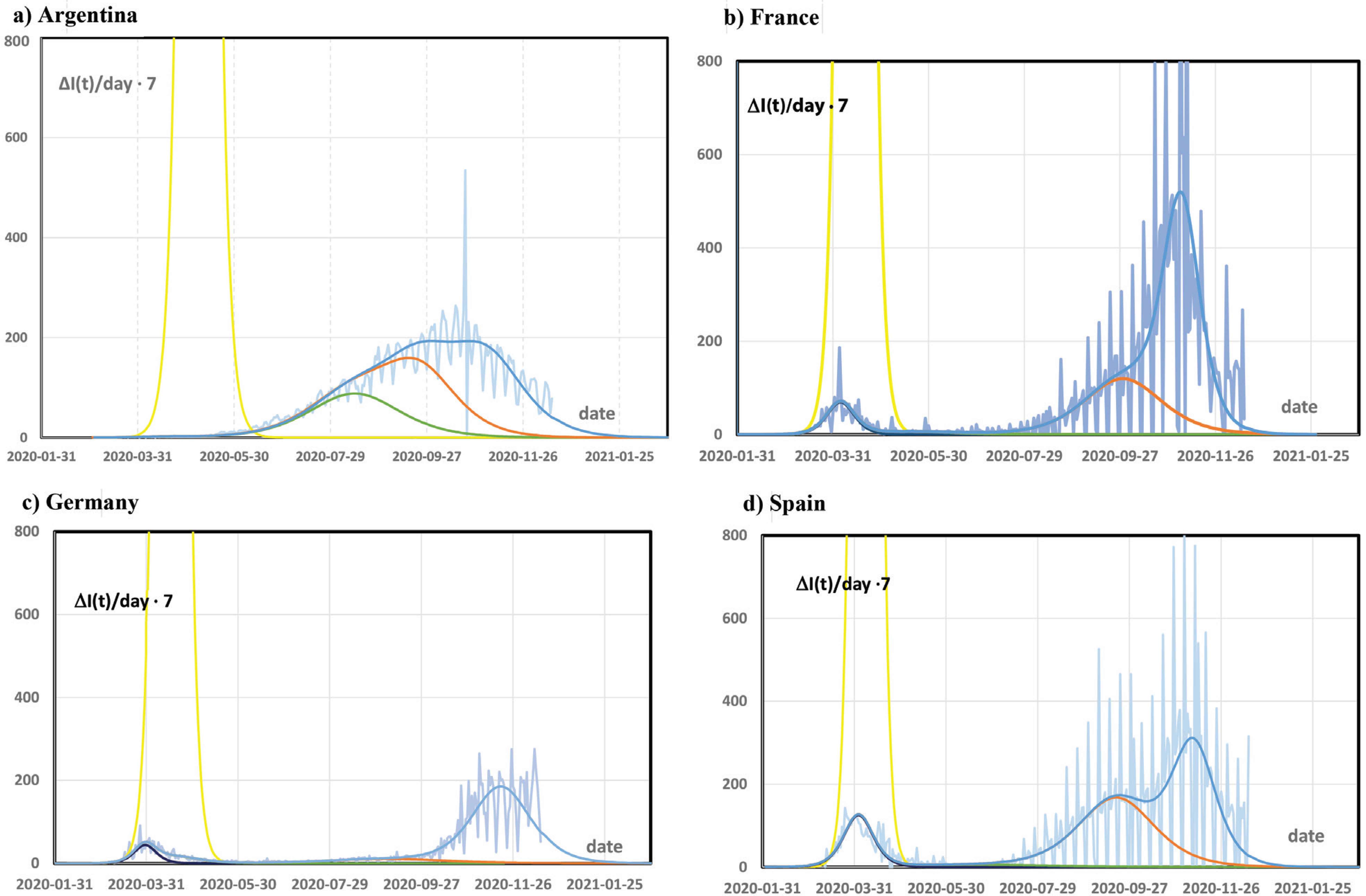
Infection rate per 100,000 persons per week. The vertical axis directly compares with the numbers for incidences per 100,000 persons per week as used e.g. for identifying high risk regions. Light blue: observed infection rates with strong weekly oscillations, yellow: extrapolated infection rate without physical distancing (N = 0), dark blue: small outbreak after the lock down (N = 1), green: outbreak during release (N = 2), orange: enhanced outbreak in summer/winter (N = 3), blue: enhanced second wave in autumn/spring since October (N = 4). All infection rates were calculated from the respective data for total case numbers [10] by taking the day-by-day differences and multiplying by seven.
The observed data are fitted by so far five outbreaks (Table 1, Figure 1 and Supplementary Figure S2.1):
- (1)
N = 0: The strictly exponential increase was interrupted after a few weeks in March by any form of physical distancing in all countries before a significant deviation from the exponential increase or a saturation were recognizable. I0,0 was very low, but infection could have gone to very high numbers of S0 ≈ P with short doubling times of only 2.3–3 days.
Four further outbreaks took place under conditions of physical distancing and continue independently from each other. A few weeks after the beginning t0,N, the additional case number IN(t) clearly drops below the initially exponential increase [3]. The time τN is significantly higher for N = 1–4 than for N = 0.
- (2)
N = 1: A short outbreak started end of February or beginning of March 2020 after interruption of exponential increase. This affected only a few tenth of percent of the population in Europe, and was nearly negligible in Argentina (cf. Supplementary Figure S2.1a). The outbreak had time constants and rate constants of around 6 days and 10−6, respectively. Without further outbreaks, the pandemic should have ended in June 2020 [8].
- (3)
N = 2: The N = 1 outbreak was immediately followed by a next one starting April to June. The case numbers in this time were often ascribed to a release of the Anti-Corona measures. The total number of infections only moderately increased by about 0.1% of the population in Europe. In Argentina, which had seen small impact of the N = 1 outbreak, the case number was higher, around 1%. The time scale of this outbreak is considerably longer than of the previous one (τ2,N around 20 days), but the rate constant is still of the order of 10−6 in Europe.
- (4)
N = 3, 4: After a calm period in May and June, two severe outbreaks were observed in late summer/winter and early autumn/spring without obvious origin. Both similarly overlap in Argentina, France and Spain (Supplementary Figure S2.1a, b, d). In Germany the outbreak N = 3 had small impact, (x3 = 0.2%), and therefore the rapid increase of the infection rate in October became very obvious. These two outbreaks together are a quantitative description of the “second wave”.
S3 and S4 during the second wave are significantly higher than S1, S2 immediately after the first measures in March. Thus, x3 and x4 are around 1–2%, and add up to an infection of 1.1–3% of the total population. All rate constants k2,3 and k2,4 are close to 10−7 being significantly lower than for N = 1 or 2. It may be speculated that this is related to the more general mask requirements during the second wave. The outbreak N = 3 started end of July till mid-August in the four countries considered here with a time scale of τ3 around 15–25 days similar to N = 2. N = 4 started in the first half of October 2020 very synchronously. τ4 is only around 10 days, which contributes mainly to the presently high incidences.
3. CONCLUSION
The total case numbers and infection rates are not only described as first and second wave, but by a total of five outbreaks. The small number of infected persons at the beginning typically increases by a factor of 10; the ratio SN/I0,N varying in a large range. In many cases, new outbreaks begin in parallel to previous ones, while these still generate significant infection rates. Uncorrelated outbreaks from different regions of large countries might be time-shifted with respect to each other, their superposition scrambling the data. As still outbreaks are distinguishable [3] they are obviously correlated in different areas and countries even under conditions of reduced human exchange.
The second wave occurs in a country on the southern hemisphere, Argentina, on a quite similar time scale with similar incidences as in Europe, in spite of different climate. The common theory that the second wave is due to autumn cooling may be discarded. Moreover, Spain is severely hit in spite of its mild climate in autumn. These observations leads to the speculative question, if the person to person transfer of the SARS-CoV-2 virus in aerosols is indeed the only efficient infection mechanism. As nearly all Anti-Corona measures aim at suppressing it, bypassing by another infection channel would explain their limited success.
CONFLICTS OF INTEREST
The author declares no conflicts of interest.
SUPPLEMENTARY MATERIALS
Supplementary data related to this article can be found at
REFERENCES
Cite this article
TY  - JOUR
AU  - Walter Langel
PY  - 2021
DA  - 2021/03/24
TI  - COVID-19: The Second Wave is not due to Cooling-down in Autumn
JO  - Journal of Epidemiology and Global Health
SP  - 160
EP  - 163
VL  - 11
IS  - 2
SN  - 2210-6014
UR  - https://doi.org/10.2991/jegh.k.210318.001
DO  - 10.2991/jegh.k.210318.001
ID  - Langel2021
ER  -