
Exact Solutions of the Nonlinear Fin Problem with Temperature-dependent Coefficients
- DOI
- 10.2991/jnmp.k.200923.001How to use a DOI?
- Keywords
- Fin equation with variable coefficients; Lie symmetries; λ-symmetries; boundary-value problems; exact solutions; linearization methods; Lagrangian and Hamiltonian
- Abstract
The analytical solutions of a nonlinear fin problem with variable thermal conductivity and heat transfer coefficients are investigated by considering theory of Lie groups and its relations with λ-symmetries and Prelle-Singer procedure. Additionally, the classification problem with respect to different choices of thermal conductivity and heat transfer coefficient functions is carried out. In addition, Lagrangian and Hamiltonian forms related to the problem are investigated. Furthermore, the exact analytical solutions of boundary-value problems for the nonlinear fin equation are obtained and represented graphically.
- Copyright
- © 2020 The Authors. Published by Atlantis Press B.V.
- Open Access
- This is an open access article distributed under the CC BY-NC 4.0 license (http://creativecommons.org/licenses/by-nc/4.0/).
1. INTRODUCTION
Fins are used in many engineering applications such as compressors, cooling of computer processor, and air-cooled craft engine in air conditioning in industry to increase the heat transfer from surfaces and they are frequently used to enable the heat loss from a heated wall. In the case of variable heat transfer coefficient and constant thermal conductivity, the analysis of the fin problem can be studied for the different cases of these dependent coefficients. If the heat transfer coefficient is a function on spatial coordinate and then it affects local temperature difference between the fin surface and the encompassing fluid. In some situations, the thermal conductivity may not be constant and it depends on temperature. This means that enormous temperature difference can be seen along the fin.
From the mathematical point of view, to obtain the exact solutions of nonlinear fin equation with temperature-dependent thermal conductivity and heat transfer coefficient is not straightforward because of the nonlinearity of the problem. The associated fin problem is given in the following dimensional form [19]
Alternatively, one can rewrite Eq. (1.5) as
In the literature, there are some studies devoted to the analysis of fin performance due to its important applications in engineering. Aziz [2] and Aziz and Enamul Hug [3] deals with perturbation method and obtains a closed-form solution for a straight convective fin with temperature-dependent thermal conductivity. Lesnic [21] Lesnic and Heggs [22] takes into account the Adomian’s decomposition method to determine temperature distribution within a straight fin with temperature-dependent heat transfer coefficient. Dulkin and Garasko [11] obtain recurrent direct solution using the inversion of the closed form solution. Sohrabpour and Razani [39] consider a method of temperature correlated profiles to obtain the solution of the optimum convective fin when thermal conductivity and heat transfer coefficients are functions of temperature. They emphasize that the effect of temperature dependence of heat transfer coefficients is important in the design of optimum fins. Khani et al. [17] compares Adomian’s decomposition method, homotopy perturbation method, and homotopy analysis method in optimizing fin performance. Zhou [43] takes into consideration differential transformation method, which based on the Taylor series expansion. Joneidi and Rashidi [15,8] present differential transformation method to obtain the efficiency of convective straight fins with temperature-dependent thermal conductivity. Lesnic [21] and Lesnic and Heggs [22] uses decomposition method, and Taylor series method used by Kim and Huang [18]. In addition, Kim et al. [19] consider the same problem by linearizing the fin equation and obtain an approximate solution.
It is a fact that theory of Lie symmetry groups is one of the most important solution methods for differential equations in the literature [16,13,12,33,32,41,42,20,31,30,27,40,14,1,35–37,34]. Specially, in the case of nonlinear differential equations, one may transform the differential equation into another equation with known solutions. Generally, transformed equations considered in the literature are linear equations. The first linearization problem for ordinary differential equation is carried out by Lie [23] indicating that a second-order ordinary differential equation is linearizable by a change of variables if and only if the equation is of the form
It is known that a second-order ordinary differential equation of the form (1.9) has first integrals, integrating factors and λ-symmetries developed by Muriel and Romero [24–26]. In recent years, some studies on the linearization through transformation involving nonlocal terms are carried out [10]. For the case of investigation of λ-symmetries of differential equations, it is possible to consider a feasible algorithm that can be applied to nonlinear differential equation of the form (1.9).
Alternatively, there is another approach called Prelle–Singer (PS) developed by Prelle and Singer [38] for analysis of first-order ordinary differential equations in the literature. PS method is based on the fact that if a given system of first-order ordinary differential equation has a solution in terms of elementary functions and then the method ensures that its solution can be found. Later Duarte et al. [9] reconstructs the technique and applies it to second-order ordinary differential equation. Their approach is based on the conjecture that if an elementary solution exists for the given second-order differential equation then there exists at least one elementary first integral. Recently, this theory is generalized to obtain general solutions without any integration and the generalized theory for the higher-order ordinary differential equations is introduced [5]. Additionally, first integrals of fin equation by linearization methods are studied and it is shown that a first integral of the associated differential equation can be obtained by using linearization methods [29]. Based on the Noether theorem, on the other hand, first integrals of an differential equation can be obtained with the method called λ-symmetry. In fact, there is a mathematical relation between λ-symmetries and PS procedure, which have been considered in literature [28,5–7]. In this study, we study novel exact invariant solutions and some solutions of boundary-value problem related to nonlinear fin equation by symmetry group-related approaches.
This study is organized as follows. In Section 2, some fundamental definitions and theorems related to the mathematical approaches are presented. In Section 3, λ-symmetries, associated first integrals, and integrating factors of the nonlinear fin equation are discussed. Additionally, exact solutions for some boundary-value problems are obtained by using the first integrals. This section also includes different cases corresponding to different choices of thermal conductivity and heat transfer coefficients. In Section 4, the generalized PS method is applied to fin equation and Lie point symmetry, first integral, λ-symmetry, integrating factor, and Lagrangian–Hamiltonian function are obtained and exact solutions for some boundary-value problems are introduced. Section 5 introduces novel solutions and results for boundary-value problems related to fin equation having physical meaning for a specific form of the thermal conductivity and some results are represented graphically.
2. PRELIMINARIES
Let us consider a second-order ordinary differential equation of the form [26]
First, solution of Eq. (2.3) gives α (θ, x) = –a2(θ, x). By substituting α into Eqs. (2.4) and (2.5), one can obtain the following differential relations
Hence, one can conclude that equations of the form (2.1) with the corresponding system (2.3)–(2.5) admit the solution for (α0, β0) such that α0 = a2. It is a fact that the coefficients of Eq. (2.1) must satisfy one of the two following alternatives: if S1 = 0, then S2 should be zero which defining by following relations
Based on these new definitions [26], the following two different cases can be considered:
Case 1: If S1 = 0, then S2 must be equal to zero.
Case 2: If S1 ≠ 0, the functions S3 and S4 must be zero.
Thus, it means that one can obtain λ-symmetry for the equation of the form (2.1) by taking into account the functions α and β. Now we examine the solutions of function β under the following different cases:
Case I: In this case, S1 and S2 are equal to zero. Then for this situation, we solve the following differential equation
Then β function is found as
Finally, we find λ-symmetry in the following form
Case II: For S1 ≠ 0, S3 and S4 must be zero. Then, we have β = S2/S1 and λ-symmetry is found by
Theorem 2.1.
[26] We consider an equation of the form (2.1) and let S1, S2, S3, and S4 be the functions defined by (2.8)–(2.11). The equation is such that either S1 = S2 = 0 or S3 = S4 = 0 if and only if ∂θ is a λ-symmetry of (2.1) for some
2.1. Prelle–Singer Approach
To introduce the Prelle–Singer (PS) approach [9], let us consider the equation
By adding a differential form of
The PS method is based on finding a function S such that the differential form (2.19) is proportional to the differential form
The existence of the functions S, I, and R satisfying (2.20) implies that
The compatibility conditions for (2.21) yield
From Eq. (2.24), we identify conjugate momentum as
3. λ-SYMMETRIES AND ASSOCIATED FIRST INTEGRALS OF THE FIN EQUATION
In the literature, the first integrals based on the linearization methods and Sundman transformation pair for nonlinear fin equation (1.6) are investigated in the study [29].
Remark 3.1.
In the study [29], first integrals of the form
In this study, λ-symmetries are studied based on linearization methods. It is a fact that one can characterize a second-order ordinary differential equation that can be linearized by means of nonlocal transformations. This characterization is given in terms of the coefficients of the equation and determines a second-order ordinary differential equation that admits λ-symmetries. There is a systematic method to find the λ-symmetries, which are used to reduce the order of differential equation. Hence, a second-order ordinary differential equation can also be integrated by a unified procedure based on λ-symmetries. For this purpose, let us assume that the equation of the form (2.1) admiting the vector field v = ∂θ by having λ-symmetry of the form
Then, we have the following propositions:
Proposition 3.1.
If S1 = S2 = 0, then there is a following relation between thermal conductivity coefficient k(θ) and heat transfer coefficient h(θ) of fin equation (1.6) of the form
where
Proof. From the equation (1.6), we have
Hence, the integration with respect to θ gives
Proposition 3.2.
Let’s S1, S2, S3, and S4 be the functions defined by (2.8)–(2.11). The relation S1 = S2 = 0 is valid if and only if ∂θ is a λ-symmetry of the form
Proof. First of all, the substitution of f(x) = σ into (2.12) yields the following differential equation of the form
The solution of the equation gives
It is a fact that there is an important relation among the λ-symmetries, the integrating factors, and the first integrals of second-order ordinary differential equation (3.10) [24,25]. To see this mathematical relation, let us consider a second-order differential equation of the form
In terms of A, a first integral of (3.11) is any function in the form of
Hence, one can determine first integrals from λ-symmetries by following steps:
- 1.
Find a first integral
where υ[λ,(1)] is the first-order λ-prolongation of the vector field υ. - 2.
- 3.
Let G is an arbitrary constant of the solution of the reduced equation written in terms of w. Therefore,
is an integrating factor of (3.11). - 4.
The solution of
- 5.
Finally, the invariant solution can be obtained by this first integral.
3.1. Invariant Solutions by using λ-Symmetries
In this part, we determine exact invariant solutions of nonlinear fin equation using λ-symmetries for different forms of heat transfer coefficient h(θ) as a classification.
Case 1: For the function h(θ) = eθ, λ-symmetry of (1.6)
To obtain an integrating factor associated to λ-symmetry, we find a first-order invariant
And taking derivative of (3.19) with respect to x gives
The use of
To find the integrating factor, above equation is written in terms of G as
The conserved form of this equation is given by
The integration of the above equation yields the invariant solution
Case 2: For the function h(θ) = θ, we have
Substituting λ in (3.14), function w is written as
Using same procedure, integrating factor becomes
Thus, the invariant solution is
Case 3: The function h(θ) = hθβ, β ≠ 1 gives λ-symmetry as
Thus, the exact analytic solution of nonlinear fin equation (1.6)
Case 4: Function h(θ) = hθβ, β ≠ −1 gives λ-symmetry as
Finally, the exact analytic solution of nonlinear fin equation (1.6) for this case is
Case 5:
If one can write ω function as
Finally, the exact solution of the fin equation (1.6)
Case 6: As the last case, for
3.2. Exact Solutions of Boundary-value Problems
The exact solutions of boundary-value problems can be obtained by using the tip and the base boundary conditions given by (1.7) and (1.8) related to the nonlinear fin problem (1.6). In the previous subsection, we obtain invariant solutions for fin equation including two arbitrary constant. Whereas by using boundary conditions, we determine these arbitrary constants and then exact solution of boundary-value equation for different cases as below.
Case 1: For the function h(θ) = eθ, the exact solution is found in (3.27). To determine the integration constants, namely c1 and c2, firstly, the base condition (1.8) is applied to (3.27) to find c2 = 2e. And then if the tip condition (1.7) is applied to (3.27) and then the other constant c3 is determined as
As a result, the solution of boundary-value problem is given by
Case 2: For the function h(θ) = θ, the invariant solution is given in (3.32). Now, we determine these constants by using boundary conditions. The base and the tip conditions yield c2 = 1 and
Case 3: The invariant solution is found in (3.37) for the function h(θ) = hθβ, β ≠ 1. Similarly, by using base condition (3.37), the constant c2 is found as c2 = 1. Then, the tip condition is applied to yield
4. THE EXTENDED PRELLE–SINGER METHOD AND λ-SYMMETRY
In this section, we consider first integrals, corresponding Lagrangian and Hamiltonian forms and exact solutions of fin problem by considering the extended PS method [9] and its the mathematical relation with λ-symmetry [26] as a different approach from the mathematical point of view.
4.1. First Integrals and Associated Lagrangian and Hamiltonian
To obtain the first integral, Lagrangian, and Hamilton functions of fin equation, let us rewrite Eq. (1.6) by using the relation (3.11) as follows
If Eq. (4.1) has a first integral
The substitution of Eq. (4.2) into the formula
The comparison of the equations given by (4.2) and (4.4) provides the following relations
Besides, the use of the compatibility conditions, namely Ixθ = Iθ,
First of all, let us consider time-independent first integral case, that is Ix = 0. Accordingly, one can easily find null function S from the first equation in (4.5) of the form
By substituting S into Eq. (4.7), we get
In fact, Eq. (4.12) is a first-order linear partial differential equation and in order to search an explicit solution for Eq. (4.12), one can assume the integrating factor R of the form
One can easily check that the functions R (4.17) and S (4.11) satisfy Eqs. (4.6)–(4.8). The associated first integral from Eq. (4.9)
Then the corresponding Lagrangian is
4.2. λ-Symmetries Determined from Lie Point Symmetries
The relation between λ-symmetries and Lie point symmetries for determination of integrating factors and first integrals of a second-order ordinary differential equation is important from mathematical point of view, based on fact that if Lie point symmetries of an equation are known and then one can construct λ-symmetries from them. For this purpose, firstly, we suppose that an equation has Lie symmetries, then determine λ-symmetries and find corresponding first integrals by using relation between the null function S and λ-symmetries.
Remark 4.1.
In the study [33], Lie symmetries and associated λ-symmetries are investigated and then the invariant solutions are determined. However, in this current study, we consider not only Lie point symmetries and related λ-symmetries but also the mathematical relation between λ-symmetries and PS method to determine invariant solutions.
Proposition 4.1.
If λ-symmetries are obtained from Lie symmetries and then the integrating factors of the equation can be determined from these λ-symmetries.
Proof. Now, we first follow an algorithm that gives λ-symmetries from Lie symmetries. For this purpose, let us consider the following second-order ordinary differential equation
Let the vector field of Eq. (4.23) be in the form of
Thus, λ-symmetries of second-order differential equation (4.23) can be obtained directly by using Lie symmetries of the same equation. Secondly, let
If ∂θ is assumed to be a λ-symmetry of (4.23) and
Consequently,
Proposition 4.2.
Suppose that v = ∂θ is a λ-symmetry. If I is a first integral of (4.23), then
The first equation in (4.32) says that v = ∂θ is a λ-symmetry for λ = −S. By writing the second and third equations of λ = −S (4.32) in terms of λ we obtain μ = −R. This reveals a role of λ = −S on the integration of Eq. (4.23), if we add
Now, we apply this algorithm to the fin equation to obtain nontrivial λ-symmetries.
Proposition 4.3.
Using compatibility condition, one-parameter Lie point symmetry of fin equation such that
Proof. For the function ϕ defined by (4.1), the operator A (4.24)
It means that fin equation has only one-parameter of symmetry group. Thus, if we substitute functions ξ and η (4.35) into (4.34), the expression
In fact, it is possible to show that S (4.37) and R (4.42) satisfy Eqs. (4.6)–(4.8). Furthermore, one can determine canonical conjugate momentum related with first integral (4.40)
And the corresponding Lagrangian
5. A SPECIAL APPLICATION
In this section, the thermal conductivity in nonlinear fin equation is considered as a linear function of temperature as a special application having physical meaning in the literature (see [19] and [18]) as
In addition, Eq. (5.2) is separated according to the power of derivatives with respect to θ to obtain determining equations in the following form
The solution of the second determining equations gives
Secondly, by taking the thermal conductivity k(θ) as a linear function of temperature as in (5.1) and by substituting (5.8) into (5.2), all coefficients a(x), b(x), c(x), and d(x) are determined. As a result, the heat transfer coefficient as a power function of temperature and associated infinitesimal functions will be as below
For this case, the thermal conductivity and the heat transfer coefficient are
First, the characteristic equation
By evaluating A(w), one can have
If G(x, w) is expressed in terms of
If the functions R and S are substituted into Eqs. (4.6)–(4.8), one can check that S and R also satisfy these equations. First, from the solution of Eq. (5.19), the invariant solution
Finally, the solution of boundary-value problem is written as
Figure 1 and Figure 2 show the evaluation of the effects of design parameters on temperature for some values of β parameter.
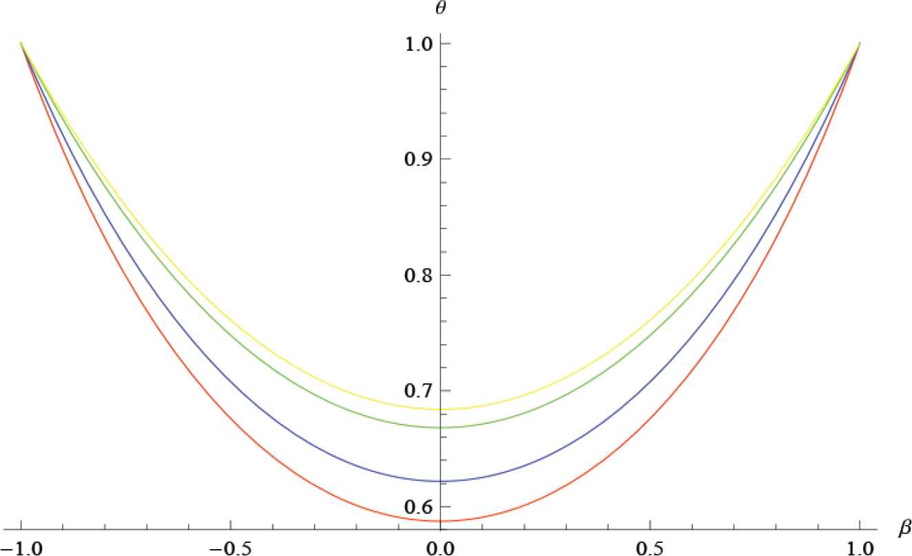
Plot of the temperature (5.23) of the fin for different values of β.
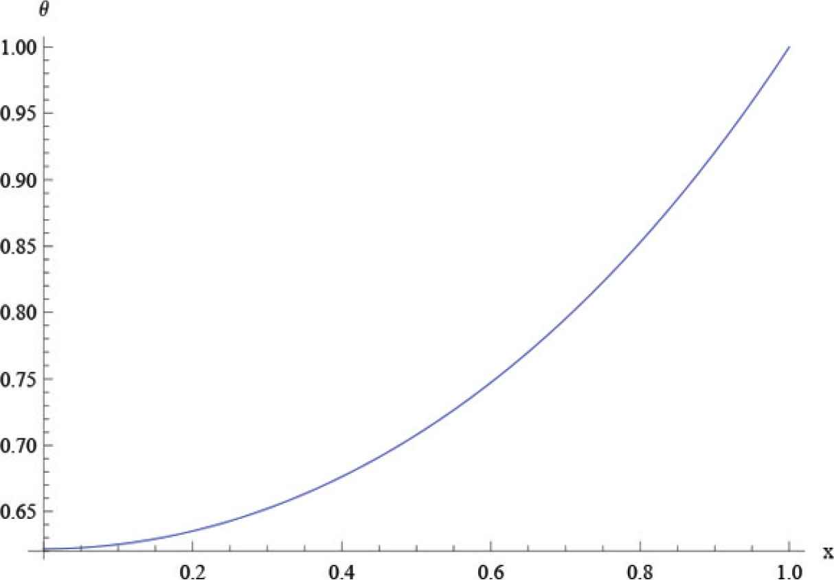
The change of the temperature (5.23) of the fin for β = −0.2.
As another case, we consider that c2 = 1 and other constants are zero. For this case, the infinitesimals take the form
It is clear that the associated thermal conductivity and the heat transfer coefficients are
And the characteristic equation is
The λ-symmetry is obtained as
The null function S, which is defined by PS method, is
The use of previous same procedure yields the integrating factor as
It can be shown that R and S also satisfy compatibility condition. The corresponding exact invariant solution can be determined as
In addition, the application of boundary conditions gives
Finally, one can write the analytical solution of boundary-value problem as below
Figure 3 and Figure 4 show the evaluation of the effects of design parameters on temperature for some values of β parameter.
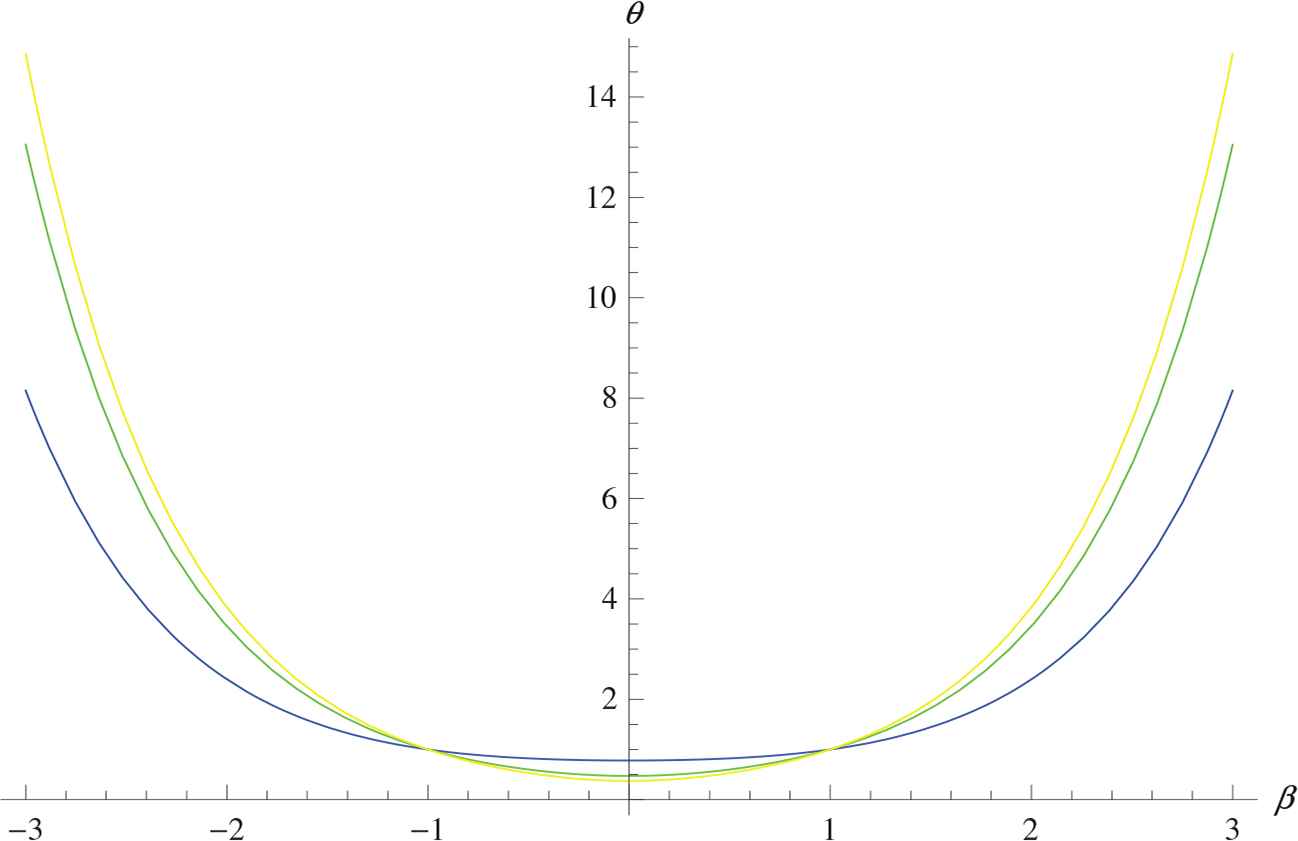
Plot of the temperature (5.32) of the fin for different values of β.
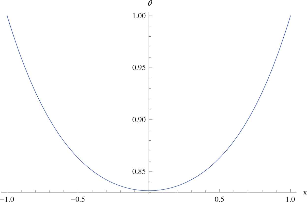
The change of the temperature (5.32) of the fin for β = −2.5.
6. CONCLUSION
In this study, a nonlinear fin problem in a one-dimensional model describing heat transfer with temperature dependent thermal conductivity and heat transfer coefficient is investigated by using the symmetry-transformation approach including λ-symmetries and Lie point symmetries. First, we analyze first integrals, integrating factor, and exact solutions of nonlinear fin equation by considering λ-symmetries and Lie point symmetries. Here, we suppose thermal conductivity and heat transfer coefficient as variable functions of temperature. From the mathematical point of view, it can be said that this problem is highly nonlinear. For different heat transfer coefficient and thermal conductivity functions, we obtain first integrals, λ-symmetries, and integrating factors. Finally, we determine the corresponding invariant solutions for each case. In addition, we determine time-independent first integrals by using the modified Prelle–Singer approach and present the mathematical relations between these approaches. Moreover, we construct Lagrangian and Hamiltonian functions from time independent first integrals and transformed corresponding Hamiltonian forms to standard Hamiltonian forms. Via the Prelle–Singer procedure, the explicit solutions satisfying all three determining equations (4.6)–(4.8) are determined. In this study, a specific ansatz forms to determine the null forms S, and integrating factor R is considered. The results related to this ansatz validate with the solution for the special case and a satisfactory accuracy is observed.
Furthermore, we investigate not only invariant solutions but also solutions of boundary-value problems related to fin problem. After obtaining the invariant analytical solutions, the boundary conditions at the tip and at the base of the fin are applied. For special choices of thermal conductivity and heat transfer coefficient functions, the solutions of boundary-value problem are determined for different cases. Furthermore, a special application with physical meaning is considered. In this case, the thermal conductivity in the nonlinear fin equation is taken as a linear function of temperature and the heat transfer coefficient is determined as a power function of temperature, which are functions considered usually for analysis of fin problem and for these special types of functions, numerical and approximate analytical solutions are carried out in the literature. However, in this current study, we represent the exact analytical solutions for the same problem. Further, to obtain the exact invariant solution and associated solution of boundary-value problem, the cases c1 = 1 and c2 = 1 are only considered. It is clear that the other types of analytical solutions can be investigated for other group parameters. In addition, the graphical interpretations of the solution as temperature function with respect to different values of a nondimensionalized parameter β and space variable x are represented.
CONFLICTS OF INTEREST
The authors declare they have no conflicts of interest.
REFERENCES
Cite this article
TY  - JOUR
AU  - Özlem Orhan
AU  - Teoman Özer
PY  - 2020
DA  - 2020/12/10
TI  - Exact Solutions of the Nonlinear Fin Problem with Temperature-dependent Coefficients
JO  - Journal of Nonlinear Mathematical Physics
SP  - 150
EP  - 170
VL  - 28
IS  - 1
SN  - 1776-0852
UR  - https://doi.org/10.2991/jnmp.k.200923.001
DO  - 10.2991/jnmp.k.200923.001
ID  - Orhan2020
ER  -