
Linearizable boundary value problems for the elliptic sine-Gordon and the elliptic Ernst equations
- DOI
- 10.1080/14029251.2020.1700649How to use a DOI?
- Keywords
- Boundary value problem; elliptic equation; Riemann–Hilbert problem
- Abstract
By employing a novel generalization of the inverse scattering transform method known as the unified transform or Fokas method, it can be shown that the solution of certain physically significant boundary value problems for the elliptic sine-Gordon equation, as well as for the elliptic version of the Ernst equation, can be expressed in terms of the solution of appropriate 2 × 2-matrix Riemann–Hilbert (RH) problems. These RH problems are defined in terms of certain functions, called spectral functions, which involve the given boundary conditions, but also unknown boundary values. For arbitrary boundary conditions, the determination of these unknown boundary values requires the analysis of a nonlinear Fredholm integral equation. However, there exist particular boundary conditions, called linearizable, for which it is possible to bypass this nonlinear step and to characterize the spectral functions directly in terms of the given boundary conditions. Here, we review the implementation of this effective procedure for the following linearizable boundary value problems: (a) the elliptic sine-Gordon equation in a semi-strip with zero Dirichlet boundary values on the unbounded sides and with constant Dirichlet boundary value on the bounded side; (b) the elliptic Ernst equation with boundary conditions corresponding to a uniformly rotating disk of dust; (c) the elliptic Ernst equation with boundary conditions corresponding to a disk rotating uniformly around a central black hole; (d) the elliptic Ernst equation with vanishing Neumann boundary values on a rotating disk.
- Copyright
- © 2020 The Authors. Published by Atlantis and Taylor & Francis
- Open Access
- This is an open access article distributed under the CC BY-NC 4.0 license (http://creativecommons.org/licenses/by-nc/4.0/).
1. Introduction
A novel method for analyzing initial-boundary value problems for integrable nonlinear evolution PDEs in one spatial dimension was introduced in 1997 [13] (see also [14]) and was further developed by several authors (see for example [4, 5, 17, 18]). This method, known as the unified transform or Fokas method, is based on ideas of the inverse scattering transform and it expresses the solution q(x,t) of a given initial-boundary value problem in terms of the solution of a matrix Riemann–Hilbert (RH) problem. This problem involves an explicit (x,t)-dependence in the form exp[ikx − iω(k)t], where ω(k) is the dispersion relation of the associated linearized evolution PDE, as well as certain functions of the spectral parameter k ∈ ℂ, called spectral functions. The main difficulty with initial-boundary value problems, as opposed to initial value problems, is that whereas in the latter case the spectral functions are defined in terms of the given initial conditions, in the former case, the spectral functions, in addition to the given initial and boundary conditions, also involves unknown boundary values. These unknown functions can be characterized in terms of the given data via the so-called global relation. Significant progress in the analysis of the global relation was achieved in [2] and [16], where it was shown that the unknown boundary values can be expressed explicitly in terms of the given data and certain eigenfunctions; however, these eigenfunctions do depend on the unknown boundary values, thus the problem of expressing the unknown boundary values in terms of the given data remains nonlinear.
It was shown in [14] that for a particular class of boundary conditions, called linearizable, it is possible to bypass the above nonlinear step and express the spectral functions explicitly in terms of the given data; linearizable boundary value problems (BVPs) are discussed in [3, 6, 7, 15, 19, 22].
The new method was implemented for integrable nonlinear elliptic PDEs in two dimensions in [20] (see also [30,31]) and [23–25]; namely in these papers the sine-Gordon equation formulated in a semi-strip and the elliptic Ernst equation formulated in a domain representing the exterior of a thin rotating disk were analyzed. It is interesting that for these PDEs and these particular domains, there exist several linearizable boundary conditions. In recent years, the Fokas method has been used by many investigators for the analytical as well the numerical investigation of both linear and nonlinear elliptic PDEs, see for example [1, 8–12, 21, 26, 29, 32, 33].
In this paper the following linearizable BVPs will be analyzed:
- (a)
Let q(x,y) satisfy the elliptic sine-Gordon equation
in the semistripdepicted in Figure 1, with the Dirichlet boundary conditions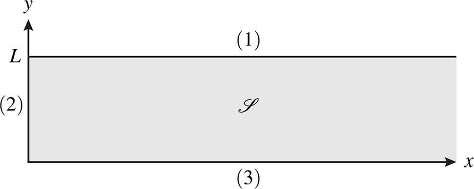 Fig. 1.
The semistrip 𝒮 used in the formulation of the BVP for the elliptic sine-Gordon equation.
where L > 0 and d ∈ ℝ are finite constants. - (b)
Let 𝒟 ⊂ ℂ denote the domain
where ρ0 > 0 is a constant, see Figure 2. Let z = ρ + iζ with ρ,ζ ∈ ℝand consider the problem of finding a function f(z) which satisfies the elliptic Ernst equation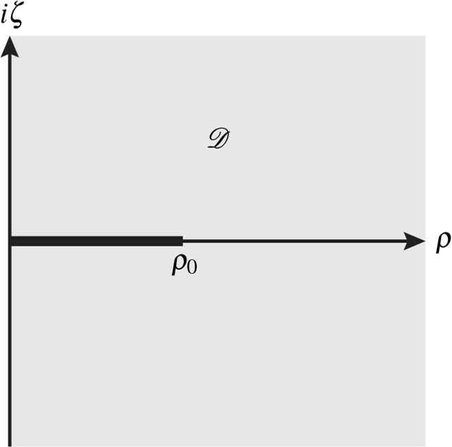 Fig. 2.
The exterior domain 𝒟 of a finite disk of radius ρ0 used in the formulation of the BVPs for the elliptic Ernst equation.
together with the following boundary conditions:where Ω ∈ ℝ is a constant and fΩ denotes the Ernst potential in a frame corotating with angular velocity Ω, see section 4. - (c)
Let f(z) satisfy the same BVP as in (b), but with the boundary condition (1.5b) replaced with
where Ωh ∈ ℝ and r1 > 0 are constants. - (d)
Let f(z) satisfy the same BVP as in (b), but with the boundary condition (1.5c) replaced with
The BVPs (b) and (c) correspond to a uniformly rotating dust disk and a dust disk rotating uniformly around a central black hole, respectively, cf. [24, 27]. In fact, the solution of the BVP formulated in (b) is the celebrated Neugebauer-Meinel disk [28] of radius ρ0 rotating with angular velocity Ω. Moreover, if one sets ρ0 = 0 in (c) (i.e. one removes the disk), then the solution of the obtained BVP is the Kerr black hole rotating with angular velocity Ωh. In the z-plane, the event horizon of this black hole stretches along the imaginary axis from −ir1 to ir1.
The problems (a)–(d) were studied in detail using the unified transform in [20], [23], [24], and [25], respectively. The purpose of this paper is to review the approaches and results of these references while emphasizing the unified nature of the approach.
2. The sine-Gordon Equation on the Semistrip
We will express the solution q(x,y) in terms of the solution of a 2 × 2 RH problem (details are given in [20]). As it was mentioned in the Introduction, this RH problem depends on certain spectral functions.
2.1. The spectral functions
The spectral functions associated with the sides (1), (2), (3) indicated in Figure 1, will be denoted respectively by
These functions are uniquely defined in terms of the following boundary values:
We assume that
For a 2 × 2-matrix A, let [A]1 and [A]2 denote the first and second columns of A, respectively. The functions a1(k) and b1(k) are defined by
The functions a2(k) and b2(k) are defined by
The functions a3(k) and b3(k) are defined by equations which are similar to (2.2) but with Q(1) replaced by Q(3).
2.2. The global relation
The spectral functions satisfy the following pair of global relations:
Theorem 2.1 ([20]).
Suppose that a subset of the boundary values {q(x,L),qy(x,L)},{q(x,0),qy(x,0)}, 0 < x < ∞, and {q(y,0),qx(y,0)}, 0 < y < L, satisfying (2.1), are prescribed as boundary conditions. Suppose that these prescribed boundary conditions are such that the global relations (2.4a) and (2.4b) can be used to characterize the remaining boundary values. Define the spectral functions {aj,bj}, j = 1,2,3, by (2.2)–(2.3). Assume that a1(k) and a3(k) do not have zeros for Imk ≥ 0.
Define M(x,y,k) as the solution of the following 2 × 2 matrix RH problem:
The function M(x,y,k) is a sectionally meromorphic function of k away from ℝ ∪ iℝ.
M satisfies the jump condition
where M = M+ for k in the first or third quadrant, and M = M− for k in the second or fourth quadrant of the complex k plane, and J is defined in terms of {aj, bj} as follows:where the functions θ, I, R are defined by
Then, M exists and is unique, provided that the H1 norm of the spectral functions is sufficiently small.
Define q(x,y) in terms of M(x,y,k) by
Then q(x,y) solves (1.1). Furthermore,
3. Linearizable Boundary Conditions for the Elliptic sine-Gordon Equation
We now concentrate on the particular boundary conditions (1.3). In this case, using the notations
In equations (3.1a) and (3.1c), the only dependence on k is through Ω(k). Thus, since Ω(−1/k)= Ω(k), it follows that the vector functions (A1,B1) and (A3,B3) satisfy the same symmetry properties. Hence,
It turns out that the vector function (A2,B2) also satisfies a certain symmetry condition, as stated in the following proposition.
Proposition 3.1.
Let qx(0,y) be a sufficiently smooth function. Then the vector solution of the linear Volterra integral equation (3.1b) satisfies the following symmetry conditions for 0 < y < L and k ∈ ℂ:
Recalling that a2(k)= A2(0,k), and b2(k)= B2(0,k), equations (3.3) immediately imply the following important relations:
In summary, the basic equations characterizing the spectral functions are:
- (a)
- (b)
- (c)
the conditions of unit determinant.
It turns out that, using these equations, it is possible to provide an explicit characterization of all the spectral functions in terms of the given constant d.
Proposition 3.2.
Assume that the functions {aj(k),bj(k)}, j = 1,2,3 satisfy the symmetry relations (3.2) and (3.5), the global relations (2.4a) and (2.4b), and the unit determinant conditions
Remark 3.1.
The two relations (3.7c) and (3.7d) are a direct consequence of the global relation and of the conditions of unit determinant. On the other hand, equations (3.7a) and (3.7b) depend on the particular symmetry properties.
Remark 3.2.
The determinant condition (3.6) with j = 1 and equation (3.7a) imply
Indeed, equation (3.6) with j = 1 implies the identity
Equation (3.9) defines the jump relation of a scalar RH problem for the sectionally analytic function defined by
Taking into consideration that a1(k) ≠ b1(k) for k ∈ ℂ+ (otherwise equation (3.6) with j = 1 is violated) it follows that the above Riemann–Hilbert problem has a unique solution
Using the fact that G(k) is an odd function, it follows that H(k) is also an odd function, hence h(−k)= e−H(k). This implies that the function h(k) defined by (3.12) satisfies the jump condition (3.9).
3.1. Spectral theory in the linearizable case
In the case of the linearizable boundary conditions (1.3), it is possible to express q(x,y) in terms of the solution of a RH problem whose jump matrices are computed explicitly in terms of the given constant d ∈ ℝ. Indeed, equations (3.7c) and (3.7d) imply that the functions R(k) and I(k) in (2.6) are given by
Thus in the linearizable case, the jump matrices involve only the ratios
Hence the jump matrices depend on the known function G/h as well as on the unknown functions
Theorem 3.1 ([20]).
Let q(x,y) satisfy equation (1.1) and the boundary conditions (1.3). Then q(x,y) is given by equations (2.7) with M replaced by
This RH problem is regular and has a unique solution.
4. The Elliptic Ernst Equation in an Exterior Disk Domain
We first consider the case of a rotating disk in the absence of a central black hole. Thus, let f (z) be a solution of the elliptic Ernst equation (1.4) in 𝒟, which satisfies the boundary conditions (1.5a) and (1.5b) together with some compatible, but otherwise arbitrary, boundary conditions along the disk.
For each z ∈ 𝒟, we let 𝒮z denote the compact Riemann surface of genus 0 defined by the equation
We view 𝒮z as a two-sheeted covering of the Riemann k-sphere endowed with a branch cut from −iz to
Proposition 4.1.
Let f (z) satisfy the Ernst equation (1.4) in the exterior disk domain 𝒟. Suppose that f satisfies the boundary conditions (1.5a) and (1.5b) and that Re f > 0 in 𝒟. The solution f(z) can be expressed in terms of the Dirichlet and the Neumann boundary values on the disk as follows:
- 1.
Use the disk boundary values of f to define the 2 × 2-matrix valued one-forms WR(ρ ± i0,k) and WL(ρ ± i0,k) for 0 < ρ < ρ0 and k = ik2, 0 < k2 < ρ0,by
and - 2.
Define a function Ψ(ρ ± i0,k) for 0 < ρ < ρ0 and k = ik2, 0 < k2 < ρ0, by solving the ordinary differential equation
together with the initial conditionsas well as the following continuity condition at the rim of the disk: - 3.
Let
and define the functions F±(k),G±(k) by solving the algebraic system - 4.
Define a 2 × 2-matrix valued function D(k),k = ik2, 0 < k2 < ρ0 by
The entries of D(k) are rational functions of the entries of C(k). Define D(ik2) for −ρ0 < k2 < 0 by
- 5.
Let Φ(z,k) be the unique solution of the following RH problem:
For each z, Φ(z,·) is a map from the Riemann surface 𝒮z to the space of 2 × 2 matrices.
Φ(z,k) is an analytic function of k ∈ 𝒮z \ (Γ+ ∪ Γ−), where Γ+ and Γ− denote the coverings of Γ =[−iρ0,iρ0] in the upper and lower sheets of 𝒮z, respectively.
Across Γ+, Φ satisfies the jump condition
where Φ+ and Φ− denote the values of Φ infinitesimally to the right and left of Γ+, respectively.Across Γ−, Φ satisfies the jump condition
As k → ∞, Φ satisfies
Φ obeys the symmetries
- 6.
Find f (z) from the equation
4.1. Equatorial symmetry and the global relation
Since only a subset of the boundary values can be specified for a well-posed problem, the solution formula presented in Proposition 4.1 is not yet effective. However, for equatorially symmetric solutions whose boundary values possess a sufficient amount of symmetry (such boundary values are called linearizable), the unknown boundary values can be eliminated by using the global relation.
The elliptic Ernst equation (1.4) admits the Lax pair
We let Φ be the solution of (4.7) which satisfies the initial conditions
Proposition 4.2.
The values of Φ on the rotation axis ρ = 0 can be expressed in terms of two spectral functions F(k) and G(k),
Proposition 4.3.
Suppose that f is equatorially symmetric, i.e., that
and A± denote the values of A to the right and left of Γ, respectively.
Remark 4.1.
For the BVPs denoted by (b)–(d) in the Introduction, symmetry considerations and the assumption of uniqueness imply that the solution is equatorially symmetric.
5. Linearizable Boundary Conditions for the Elliptic Ernst Equation
For a linearizable BVP, the spectral functions F(k) and G(k) satisfy, in addition to the global relation (4.9), an additional important algebraic relation. These two algebraic relations satisfied by F(k) and G(k) yield an auxiliary RH problem for F and G with jump data formulated in terms of the known boundary values alone.
5.1. A rotating disk
Suppose f (z) is a solution of the BVP formulated in (b) of the Introduction. We will show that the boundary conditions satisfied by f are linearizable and derive an explicit expression for the solution f in terms of theta functions (see [23] for details). In this way we recover the Neugebauer-Meinel disk solutions [28].
The boundary conditions (1.5) and (1.6) involve the corotating Ernst potentials fΩ and fΩh, which are defined as follows. Outside a stationarily rotating axisymmetric body, the Einstein field equations are equivalent to the elliptic Ernst equation (1.4). Indeed, in canonical Weyl coordinates the exterior gravitational field of such a body is described by the line element
The Ernst equation retains its form in the corotating system and fΩ denotes the corresponding Ernst potential.
Proposition 5.1.
Suppose that fΩ is constant along the disk. Let f0 := f (+i0) and define B and Λ(k) by
Then the spectral functions F(k) and G(k) satisfy the relation
Combining Propositions 4.3 and 5.1 we can determine the spectral functions F and G via the solution of a 2 × 2 matrix RH problem.
Proposition 5.2.
Suppose f satisfies the BVP denoted by (b) in the Introduction. Then the spectral functions F(k) and G(k) are given by
ℳ (k) is analytic for k ∈ ℂ\Γ, Γ =[−iρ0,iρ0].
Across Γ, ℳ (k) satisfies the jump condition
where ℳ+ and ℳ− denote the values of ℳ to the right and left of Γ, respectively, and 𝒮 (k) is defined byℳ has the asymptotic behavior
The auxiliary RH problem presented in Proposition 5.2 can be used to determine the spectral functions F and G, which can then be used to set up the main RH problem. In fact, following [27,28] we can also obtain the solution f directly by combining the main and auxiliary RH problems into a single scalar RH problem. It turns out that the solution can be expressed explicitly in terms of theta functions associated with the Riemann surface Σz of genus 2 defined by the equation
The homology basis
We denote by ωPQ the normalized Abelian differential of the third kind on Σz, which has simple poles at the points P and Q with residues +1 and −1, respectively.
Theorem 5.1.
Let ρ0,w2 > 0.a Let the function h(k) be defined by
Define the z-dependent quantities u ∈ ℂ2 and I ∈ ℝ by
Then the function
5.2. A disk rotating around a black hole
Suppose f(z) is a solution of the BVP formulated in (c) of the Introduction and let Φ(z,k) be the eigenfunction defined by (4.7) and (4.8). The boundary values (1.6) imply that Φ has simple poles at the points k = ±r1 where there regular rotation axis meets the horizon. Thus, the effect of including a central black hole is to add two bound states (which correspond to solitons) to the solution.
Let f0 := f (+i0) and f1 := f (ir1). The following four propositions are the analogs of Propositions 4.2, 4.3, 5.1, and 5.2.
Proposition 5.3.
The values of Φ on the ζ -axis can be expressed in terms of two spectral functions F(k) and G(k) as
Proposition 5.4.
The spectral functions F(k) and G(k) defined in Proposition 5.3 satisfy the global relation
Proposition 5.5.
The spectral functions F(k) and G(k) satisfy the relation
Proposition 5.6.
Suppose f satisfies the BVP denoted by (c) in the Introduction. Then the spectral functions F(k) and G(k) are given by
ℳ (k) is analytic for
Across Γ, ℳ (k) satisfies the jump condition (5.3), where 𝒮 (k) is defined by
ℳ has the asymptotic behavior ℳ (k)= σ1 + O(k−1) as k → ∞.
The entries of ℳ have simple poles at k = r1 and k = −r1. The associated residues are given by
whereand d+/dζ denotes the right-sided derivative.
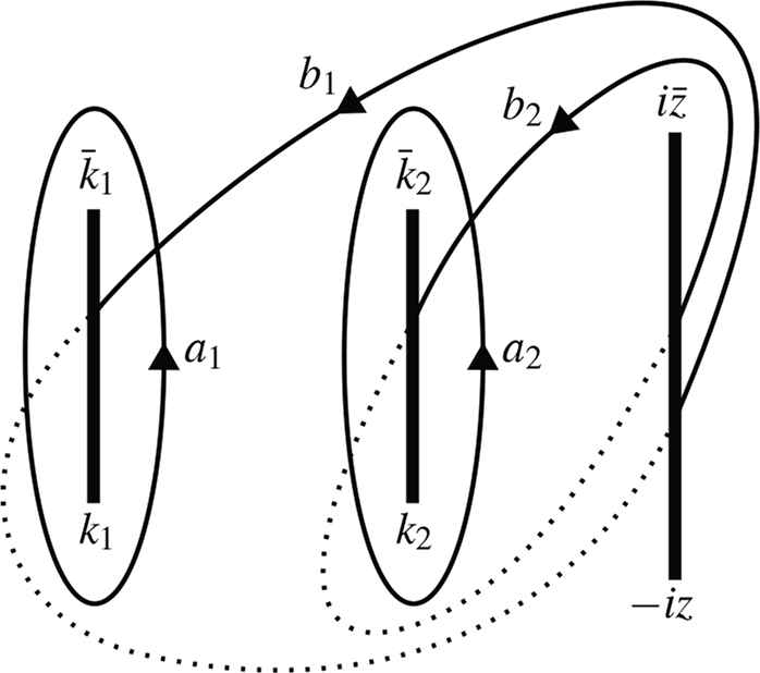
It turns out that the main and auxiliary matrix RH problems can be combined into a single scalar RH problem formulated on the Riemann surface Σz of genus 4 consisting of all points (k,y) ∈ ℂ2 such that
We let γ denote the contour on Σz which projects to the contourb
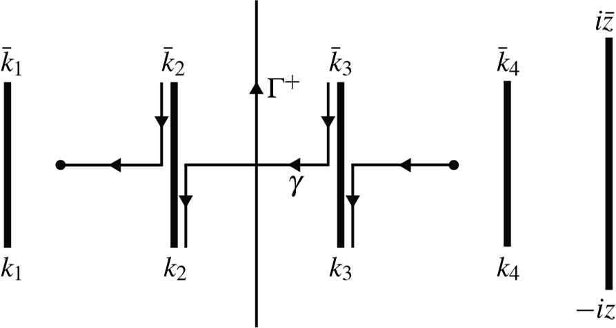
The genus 4 Riemann surface Σz defined in (5.16) presented as a two-sheeted cover of the complex k-plane together with the contours γ and Γ+.
For simplicity, we assume that
Using notations analogous to those used in Theorem 5.1. we can state the following result.
Theorem 5.2 ([24]).
Let ρ0, r1, w2, w4 be strictly positive numbers such that (5.18) holds; the requirement that the solution be singularity-free imposes further restrictions on these parameters, see [24]. Let the function h(k) be defined by
Define the z-dependent quantities u ∈ ℂ4 and I ∈ ℝ by
Then the function
5.3. A disk with a Neumann condition
Suppose f (z) is a solution of the BVP formulated in (d) of the Introduction for some choice of the parameters ρ0 > 0 and Ω > 0 such that 2Ωρ0 < 1. Then the following analogs of Propositions 5.1 and 5.2 are valid (see [25] for details).
Proposition 5.7.
Suppose that ∂ζ fΩ = 0 on the disk. Then the spectral functions F(k) and G(k) satisfy the relation
Proposition 5.8.
Suppose f satisfies the BVP denoted by (d) in the Introduction. Then the spectral functions F(k) and G(k) are given by
ℳ (k) is analytic for k ∈ ℂ\Γ.
Across Γ, ℳ (k) satisfies the jump condition (5.3), where 𝒮 (k) is defined by
ℳ has at most logarithmic singularities at the endpoints of Γ.
ℳ has the asymptotic behavior ℳ (k)= σ1 + O(k−1) as k → ∞.
The solution of the auxiliary RH problem of Proposition 5.2 yields the following explicit formulas for F and G, which can be used to set up the main RH problem:
Furthermore, by combining the main and auxiliary RH problems into a single scalar RH problem, the solution f can be expressed in terms of theta functions associated with the family of Riemann surfaces Σz of genus 1 defined by
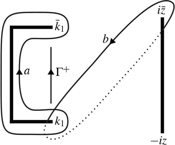
The homology basis {a,b} on the Riemann surface Σz of genus g = 1 defined in (5.22) and the contour Γ+.
Theorem 5.3 ([25]).
Let ρ0 > 0 and Ω > 0 be such that 2Ωρ0 < 1. Define the z-dependent quantities u ∈ ℂ2 and I ∈ ℝ by (5.7), where the integrals are contour integrals on the genus 1 surface Σz defined in (5.22) and h(k) is given by (5.21). Then the function f (z) defined by (5.8) satisfies the BVP denoted by (d) in the Introduction with the prescribed values of ρ0 and Ω.
Acknowledgments
ASF acknowledges support from the Guggenheim foundation and from the EPSRC in the form of a senior fellowship. JL acknowledges support from the Göran Gustafsson Foundation, the Ruth and Nils-Erik Stenb¨ack Foundation, the Swedish Research Council, Grant No. 2015-05430, and the European Research Council, Grant Agreement No. 682537.
Footnotes
The requirement that the solution be singularity-free imposes further restrictions on these parameters, see [27]. The correspondence between the parameter w2 used here and the parameter μ in [27] is
For n complex numbers
References
Cite this article
TY  - JOUR
AU  - Jonatan Lenells
AU  - Athanassios S. Fokas
PY  - 2020
DA  - 2020/01/27
TI  - Linearizable boundary value problems for the elliptic sine-Gordon and the elliptic Ernst equations
JO  - Journal of Nonlinear Mathematical Physics
SP  - 337
EP  - 356
VL  - 27
IS  - 2
SN  - 1776-0852
UR  - https://doi.org/10.1080/14029251.2020.1700649
DO  - 10.1080/14029251.2020.1700649
ID  - Lenells2020
ER  -