1. Introduction

Let 𝒜_N denote a phase space of N-particle one dimensional dynamical system with coordinates q_i and momenta p_i, i = 1,...,N, canonical with respect to the Poisson bracket {q_i, p_j} = δ_ij. Let H = H(q, p) denote the Hamiltonian of this system, where q = (q₁,...,q_N), p = (p₁,..., p_N), i.e., q˙i={qi,H}, p˙i={pi,H}. We assume that q_i are either real or pairwise complex conjugate and the same are properties of the corresponding p_i. Let we have a function f(q, p) on 𝒜_N and let f(q − x 1, p) denote this function with all coordinates q_i shifted by a real parameter x, 1=(1,…,1)︸N. In what follows we assume that equation

The induced system is not only Hamiltonian but also integrable, as by construction it has (at least) N integrals of motion in involution.

Assume, that (q, p) ∈ 𝒜′_N, i.e., there exists exactly N real (different) solutions of the Eq. (1.1):

Taking (1.3) into account we differentiate (1.4) twice with respect to t:

One can consider (1.4) and (1.5) as system of 2N equations on 2N unknowns q and p, that are defined by means of these equations as functions of x and ẋ under condition of unique solvability of this system, that we assume below. Inserting these functions in (1.6) we prove existence of the Newton-type equations of the induced dynamical system:

The above consideration gives also scheme of solution of the Cauchy problem for the induced system. Let we are given with 2N initial data: x_i(0) and ẋ_j(0), say at t = 0, where i, j = 1,...,N. Equations (1.4) and (1.5) define values (q(0), p(0)) that belong to 𝒜′_N by definition. Then by (1.3) q_i(t) = q_i(0) + th′(p_i), p_i(t) = p_i, that after substitution in (1.1) gives M real roots x₁(t),...,x_M(t) for any t ∈ ℝ. Thus the scheme of solution of the Cauchy problem for the induced dynamical system is close to the one for integrable nonlinear PDE’s. Notice that M is not obliged to be equal to N at any moment of time, i.e., point (q(t), p(t)) is not obliged to belong to 𝒜′_N for any t.

Below we demonstrate that in spite of a trivial dynamics of the system on the phase space 𝒜, dynamics of the induced system is highly nontrivial. In particular, it demonstrates effects that can be interpreted as existence of stable bound states and even as creation and annihilation of particles.

The manuscript is organized as follows. In Sec. 2 we consider dynamical systems that appeared many years ago (see, e.g., [1], [11], [12], [13], and [14]) as systems describing the dynamics of singularities of solutions of some integrable equations (“zeros” of τ-functions). While ideology developed here is based essentially on study of the singular solutions of the Liouville equation in [12] and [13], here we consider more interesting dynamics of singularities of soliton solutions of the KdV and Sinh–Gordon equations and show that this dynamics is the induced one. In Sec. 3 we derive a new determinant formula for solutions of the well known dynamical systems: rational Calogero–Moser, [3, 4], and Ruijsenaars–Schneider, [16, 17], models. By these means dynamics of these systems also can be described as the induced one, that explicitly demonstrates their Liouville integrability. We also suggest some integrable generalizations of these models. In Sec. 4 we present some other simple examples of the induced systems given by polynomial functions f in (1.1), both in nonrelativistic and relativistic cases. Results and possible developments of the suggested technique are discussed in Sec. 5. Properties of the induced systems under consideration are displayed by means of figures carried out by package Wolfram Mathematica 11.1.

2. Dynamics of singularities of solutions of integrable differential equations

2.1. Singular solutions of the KdV equation

In this section we show that old results on dynamics of singularities of soliton solutions (singular solitons) of integrable PDE’s can be formulated in terms of induced dynamics. We start with N-soliton solution of the KdV equation 4u_t − 6uu_x + u_xxx = 0 on a real function u(t, x), where indexes denote partial derivatives. This famous equation is known to have both regular (see, e.g., [8]) and singular (see [1]) N-soliton solutions. Their generic form is given by

u(t,x)=−∂x2log det(E(t,x)+v)2,(2.1)

where E(t, x) and v are correspondingly diagonal and constant N×N-matrices,

E(t,x)=diag{εie2pi(x−ai−pi2t)},   vij=2pipi+pj.(2.2)

Here a_i, p_i, and ε_i = ±1, i = 1,...,N, are constant parameters of the solution such that Re p_i > 0 and

either Impi=0,   εi=±1,   Imai=0,or Impi≠0,  then there exists pl=p¯i,   εl=εi=±1,   al=a¯i.(2.3)

If Im p_i = 0 signs ε_i = +1 and ε_i = −1 correspond to the regular and singular solitons. Every pair of pi=p¯l with Im p_i ≠ 0 gives one line of singularity. All singularities of the solution u(t, x) are given by the zeros of determinant in (2.1): det(E(t, x) + v) = 0. Thus in generic situation we have interaction of regular and singular solitons and breathers, the latter correspond to mutually conjugate pairs of parameters. In [1] it was shown that singularities of this solution form smooth curves on (x, t)-plane. They run from minus to plus t-infinities and thus are observable at any moment of time. On the other side, the regular solitons are known to be observable outside the collision region only. Taking that asymptotic behavior of the regular and singular solitons coincides into account, we suggested (see [1]) to introduce a “charge conjugation”, i.e., to change all signs ε_i → − ε_i in (2.2). Then regular and singular solitons mutually exchange and we get world lines of particles corresponding to both, regular and singular solitons, as roots of the product

det(E(t,x)+v)det(E(t,x)−v)=0.(2.4)

Notice now that introducing functions

qi(t)=ai+pi2t,   so that q˙i=pi2,   p˙i=0,   i=1,…,N,(2.5)

we rewrite (2.4) in the form (1.1), i.e., as induced dynamical system, where

f(q,p)=det(E0+v)det(E0−v),   E0=diag{εie−2piqi(t)},(2.6)

cf. (2.2). As we mentioned in Sec. 1, this dynamical system is Hamiltonian (cf. (1.2)):

H=13∑i=1Npi3,(2.7)

with respect to the canonical Poisson bracket {q_i, p_j} = δ_ij. Moreover, the system is Liouville integrable: variables {p₁,..., p_N} are integrals of motion, and they are in involution by construction. It is easy to prove that system (1.5), (1.6) for the function f in (2.6) is solvable with respect to q_i and p_i, while not explicitly. Correspondingly, forces (i.e., the r.h.s. of (1.7)) here exist but in implicit form, so that the most descriptive characterization of this induced dynamical system is given by Eq. (1.1). In spite of trivial dependence of q_i and p_i on t, cf. (2.5), dependence of zeros x_i(t) is highly nontrivial, see Figs. 1–4.

Fig. 1.

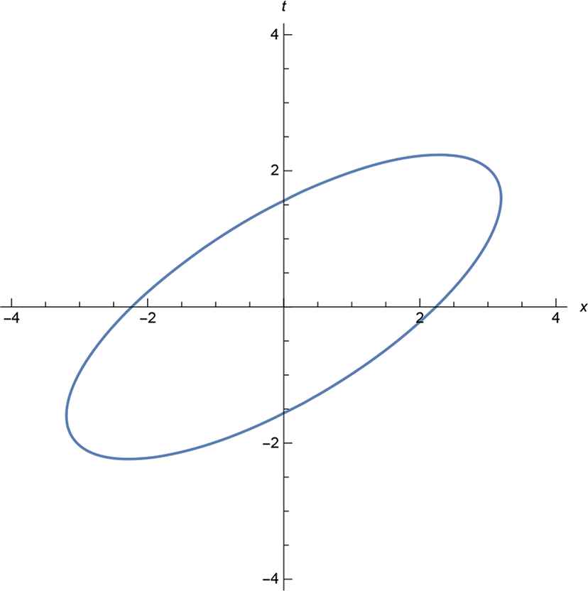
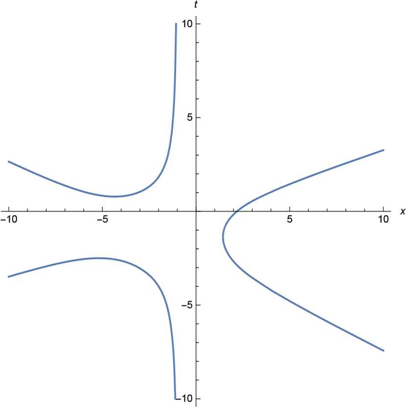
KdV: Soliton–soliton collision: ε₁ = ε₂ = 1.

Fig. 2.

KdV: Soliton–antisoliton collision: ε₁ = −ε₂

Fig. 3.

KdV: breather

Fig. 4.

KdV: soliton–breather collision

3. Rational cases of the Calogero–Moser and Ruijsenaars–Schneider models

Here we show that the rational versions of the Calogero–Moser (CM) and Ruijsenaars–Schneider (RS) models also give examples of the induced dynamics, i.e., their solutions are given as roots of Eq. (1.1) with proper choices of functions f(q, p) and h in (1.1) and (1.2). Dynamics of these models, see [3, 7, 16, 17], is given by equations

It was also proved there that, say, at t → −∞ this solutions obey asymptotic behavior

In order to prove that CM and RS systems can be written in the form (1.1), we notice that because of the translation invariance, solutions x_i(t) are roots of the characteristic equation

Now for the term (t − τ)V(τ) (see (3.3) and (3.4)) we have in the limit (3.6):

Thus solutions of the rational versions of CM and RS models are given by the roots of the equation

Eqs. (3.9)–(3.11) in their turn enables derivation of the known Lax representations for the both these models following the same lines like in [9] and [18]. In particular, we get that momenta p_i are eigenvalues of the Lax matrix (3.3).

Characteristic equation (3.9) is exactly of the form (1.1), where f(q, p) = det(Q +W), q˙i=pi and p˙i=0, i = 1,...,N, so that (q_i, p_j) are canonical variables with respect to the bracket {q_i, p_j} = δ_i,j, Hamiltonian is given by (1.2) with h(p) = p²/2 for both models. Derived representation (3.9) gives direct proof of the Liouville integrability for these models. Moreover, integrability takes place for any choice of the (off-diagonal) matrix W(p) in (3.9) that obeys conditions of solvability of the systems (1.4) and (1.5). Specific property of the CM and RS models is possibility to write down equations (3.1) and (3.2) of motion and Lax pairs explicitly, cf. discussion of this problem in Sec. 2 for the dynamics of singularities of the KdV and Sinh–Gordon equations.

4. Polynomial examples of induced dynamics

In this section we consider some simplest examples of induced dynamical systems, given by polynomial function f in (1.1):

Here C is a real constant (parameter of the system), variables q_i and p_i obey condition of reality, given in the beginning of Sec. 1 and

Such systems are more trivial then those considered in Sec. 2. Say, they do not give nontrivial phase shifts. Nevertheless, examples of N = 2 and N = 3 of these system and their relativistic analogs (see Sec. 4.2 below) demonstrate such unexpected for classical mechanics effects as creation/annihilation of particles. Notice that here we do not impose conditions of the kind Re p_i > 0 in (2.3) on variables in 𝒜_N.

4.1. Nonrelativistic case

Let us start with N = 2 in (4.1), i.e., with function f(q, p) = q₁q₂ − C/4, that also coincides with the N = 2 case of (3.9), where matrix 2×2-matrix W is off-diagonal and p-independent. Eq. (1.1) in this case sounds as

f(q−x1,p)≡(q1−x)(q2−x)−C/4=0,(4.3)

so that H=(p12+p22)/2 (cf. (1.2)). Let x₁(t) and x₂(t) denote two real solutions of Eq. (1.1). Introducing notation for the differences:

x12=x1−x2,   q12=q1−q2,(4.4)

we get

x1+x2=q1+q2,   x122=q122+C,(4.5)

so that

x˙1+x˙2=p1+p2,   p1−p2=x˙12x12q12.(4.6)

Eqs. (4.5) and (4.6) define q_i and p_i in terms of x_i and ẋ_i (cf. (1.5), (1.6)). These values, being substituted in the time derivative of (4.6) gives explicit equations of motion of the induced dynamical system, cf. (1.7):

x¨1+x¨2=0,   x¨12=Cx˙122x12(x122−C).(4.7)

It is worth to mention that under reduction to the center of mass frame, x˙1+x˙2=0, these equations coincide with the same reduction of the N = 2 case of Ruijsenaars–Schneider system (3.2).

Eqs. (4.7) are Lagrangian with

ℒ=x˙12+x˙222+Cx˙1224(x122−C).(4.8)

Variables q_i and p_i are canonically conjugate, and due to (4.5) we get {x_i, x_j} = 0. Then (4.8) enables to introduce momenta conjugate to x_i as

Pi=x˙i+(−1)i+1Cx˙122(x122−C),   i=1,2,(4.9)

so that equations (4.5) and

p1+p2=P1+P2,   p1−p2=(P1−P2)x122−Cx12

give canonical transformation from variables {x_i, P_j} to {q_k, p_l}, where i, j, k, l = 1, 2. The Hamiltonian H, being trivial in terms of the variables on 𝒜₂, equals

H=P12+P222−C(P1−P2)24x122,(4.10)

in terms of the variables on the phase space of the induced system.

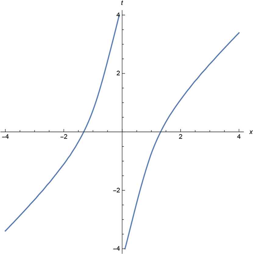
In order to show behavior of the world lines of the particles on the (x, t)-plane we consider initial problem: x_i(t)|_t=0 = a_i, ẋ_i(t)|_t=0 = v_i, where x_0,i and v_i are real initial data. These data define q_i(0) and p_i(0) by Eqs. (4.5) and (4.6). Because of the free evolution on 𝒜₂, we have that q_i(t) = q_i(0) + p_it, p_i(t) = p_i, and finally we reconstruct x_i(t) by (4.5):

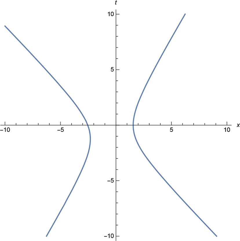
x1(t)+x2(t)=a1+a2+(v1+v2)t,(4.11)

x122(t)=(a12+v12t)2+Cv122t2a122−C,(4.12)

where we used notation for differences like in (4.4). Behavior of the roots of Eq. (4.3) on the (x, t)-plane is determined by the sign of a122−C. For the induced system with C > 0 we have in the case of a122>C that solutions x_i(t) are real for any t and x122(t)≥C>0, Fig. 5. The world lines of both particles run from minus to plus t-infinity and we have repulsion of particles in this case. But situation changes essentially if C>a122. In this case q₁₂ and p₁₂ are pure imaginary, solutions x_i(t) are real in the finite interval t₊ ≥ t ≥ t₋ of time only, where t_± are moments where the r.h.s. of (4.12) vanishes, see Fig. 6. Inside this interval C≥x122(t)>0, the background system is in 𝒜′₂, while for t = t_± we have only one solution, M = 1. For t < t₋ and t > t₊ real solutions do not exist, so M = 0 and background system belongs to 𝒜₂, but not to 𝒜′₂, so the the dynamical system (4.7) does not exist. We can interpret this behavior of the system as creation of two particles at moment t₋, where they scatter with infinite velocities. With time growing they slow down, stop and move to meet one another at t = t₊. At this moment they reach infinite velocities and annihilate. It is necessary to emphasize that, in spite of this strange evolution of the induced system, both its integrals of motion, p₁ and p₂, exist for any t.

Fig. 5.

Two particles, x122>C>0.

Fig. 6.

Two particles, C>x122>0.

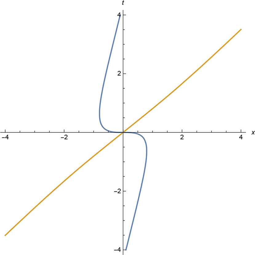
If the induced system is given by (4.3) with C < 0, we always have a122>0>C, so by (4.11), (4.12) real solutions x_i(t) exist outside of the time interval {t₋, t₊}, where x122(t)≥0, see Fig. 7 (this figure corresponds to the case where a₁₂v₁₂ < 0, for the opposite sign t-axis must be inverted). Here two particles come from infinity: they attract, speed up till infinity and bump into each other at t = t₋. At this moment they reach infinite velocities and disappear. For a period t₋ < t < t₊ induced system does not exist: the r.h.s. of (4.12) is negative. Later, at t = t₊ two particles arise with infinite velocities at some point of the x-axis. Then they slow down and blow to infinity. So we can say that at t = t₋ there is annihilation of particles and their creation at t = t₊, that looks like a bang: particles appear from nowhere. Notice that variables of phase space 𝒜₂ exist at any moment of time, independently of existence of the real solutions x_i(t). In particular, all integrals of motion exist for any t. It is necessary to emphasize that due to (4.11) and (4.12) singularities of the induced system—absence of real solutions—are movable: intervals where real solutions do not exist are defined by the initial data only. This property is analogous to the Painlevé property for integrable PDEs.

Fig. 7.

Two particles, C < 0

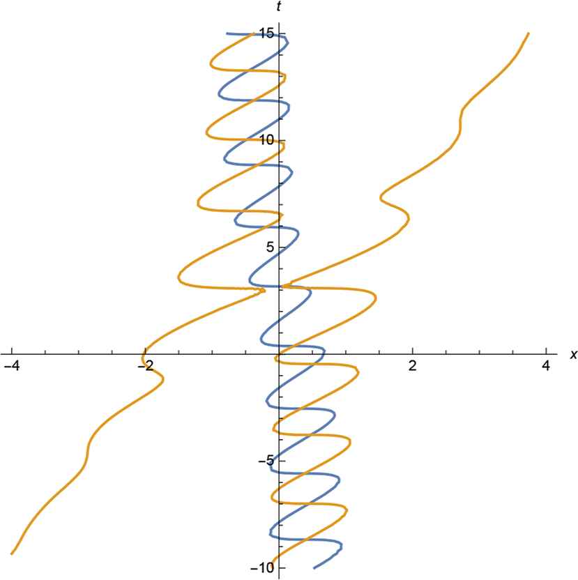
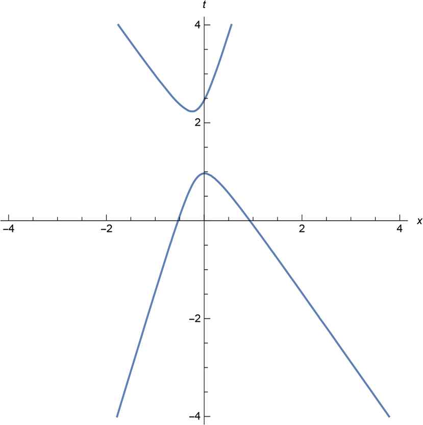
Analogously one can consider the higher values of N in (4.1). Say, on the Fig. 8 we present structure of the world lines of the system, given by N = 3 in (4.1). By no means this structure is very unexpected for dynamical systems: three particles descend from infinity, two of them annihilate and for a period induced system has only one particle (only one real solution of the equation of the third order). Nevertheless, motion of this particle is far from being free: it slows down, stops and turns back.

Fig. 8.

Three particles.

5. Concluding remarks

The idea to construct dynamical systems by means of the relationship among the zeros and coefficients of time-dependent polynomials (or possibly more general functions, for instance entire ones) is rather old, [4]. It was essentially developed later, see, e.g., [5] and references therein. This approach can be considered as a version of induced dynamics as well—the dynamics of the zeros is induced by the dynamics of the coefficients of polynomials—in fact more general than considered above. The main difference between this general approach and the notion of induced dynamical systems introduced in this article is the Liouville integrability of the latter ones. Say, coefficients of polynomial f(q − x 1, p) for dynamical system defined by (4.1) are given in terms of elementary symmetric polynomials of q_i and for a generic N evolution equations of these coefficients are neither explicit, nor give any information on integrability, in contrast to (4.2).

Induced dynamical systems of Sec. 2 were originated by the singular soliton solutions of the integrable equations, KdV and Sinh–Gordon. Thus it was natural to expect their Liouville integrability. Integrability of the CM and RS system is well known also. Unexpected result of our consideration in Secs. 2 and 3 is the existence of rich families of integrable models beyond these known ones. Thus functions f in (2.6) and (2.13) define, thanks to Eqs. (2.5) and (2.14), integrable systems not only in the case where matrix v is given by (2.2), but for an arbitrary matrix v(p). The same is valid for matrices W in Sec. 3, that are not obliged to be given by (3.11) in order to generate integrable dynamical systems by means of (3.9). Examples from Sec. 4 show that cases where forces in the r.h.s. of (1.7) are explicit are very rare, and in generic situation investigation of induced systems must be based on the description of solutions of Eq. (1.1). Properties of the induced dynamical systems (4.7) and (4.14) look to be rather strange, they are new to our knowledge and deserve further investigation. Summarizing results of Sec. 4, we see that the dynamical system on the space 𝒜_N (i.e., q˙i=p˙i, p˙i=0) plays the role of a background one. This free system exists for any t, has always N degrees of freedom and controls dynamics of the induced system. Passage in involution from subspace 𝒜′_N to 𝒜_N and vice verse leads to instant change of dimension of the induced system, recalling such quantum effects as creation/annihilation of particles. Say, in situation presented on Fig. 7 the induced dynamical system does not exist in the interval t ∈ {t₋, t₊}, while variables on 𝒜_N do exist. They include integrals of motion p_i, that coincide with integrals of the induced system. Following the famous fairy tale this effect can be referred to as “cheshirization” of our dynamical systems.

In this article we suggested notion of the induced dynamical system and proved that it gives effective method to investigation of known systems and to construction of new ones. These systems demonstrate rather nontrivial particle interactions being completely integrable by construction. Some other examples of the induced systems were presented in the preliminary version of this article, see [15]. It is also interesting to generalize consideration of the Sec. 2—dynamics of singularities of the nonlinear equations—to the case where solitons are unstable and, say, collision of two regular solitons leads to a singularity. Such soliton solutions were studied in [10], [6], and [2], in particularly for the case of the Boussinesq equation.

Acknowledgment

Author thanks G. Arutyunov, L.V. Bogdanov, F. Calogero, A.M. Liashyk, S. Ruijsenaars, and A.V. Zotov for fruitful discussions. The work is supported in part by the Russian Academic Excellence Project ‘5-100’ and by the grant RFBR # 18-01-00273.

References

[1]V.A. Arkad’ev, A.K. Pogrebkov, and M.K. Polivanov, Singular solutions of the KdV equation and the method of the inverse problem, Zap. Nauchn. Sem. LOMI, Vol. 133, 1984, pp. 17-37.
[8]S.P. Novikov, S.V. Manakov, L.P. Pitaevskii, and V.E. Zakharov, Theory of Solitons: The Inverse Scattering Method, Springer, Berlin, 1984.
[10]A.Yu. Orlov, Collapse of solitons in integrable model, Preprint IAIE, IAIE, Novosibirsk, Vol. 221, 1983.
[12]A.K. Pogrebkov and M.K. Polivanov, Interaction of particles and fields in classical theory, Soviet J. Particles and Nuclei, Vol. 14, No. 5, 1983, pp. 450-457.
[13]A.K. Pogrebkov and I.T. Todorov, Relativistic Hamiltonian dynamics of singularities of the Liouville equation, Ann. Inst. H. Poincaré Sect. AN.S., Vol. 38, No. 1, 1983, pp. 81-92.
[14]A.K. Pogrebkov and M.K. Polivanov, The Liouville and sinh-Gordon equations. Singular solutions, dynamics of singularities and the inverse problem method, Soviet Sci. Rev., Sect. C, Math. Phys. Rev., Harwood Academic Publ., Vol. 5, 1985, pp. 197-271.
[15]A.K. Pogrebkov, Induced dynamics, 2019. arXiv: 1904.09469v1
Journal
Journal of Nonlinear Mathematical Physics
Volume-Issue
27 - 2
Pages
324 - 336
Publication Date
2020/01/27
ISSN (Online)
1776-0852
ISSN (Print)
1402-9251
DOI
10.1080/14029251.2020.1700648How to use a DOI?
Copyright
© 2020 The Authors. Published by Atlantis and Taylor & Francis
Open Access
This is an open access article distributed under the CC BY-NC 4.0 license (http://creativecommons.org/licenses/by-nc/4.0/).
Cite this article
TY  - JOUR
AU  - A. K. Pogrebkov
PY  - 2020
DA  - 2020/01/27
TI  - Induced Dynamics
JO  - Journal of Nonlinear Mathematical Physics
SP  - 324
EP  - 336
VL  - 27
IS  - 2
SN  - 1776-0852
UR  - https://doi.org/10.1080/14029251.2020.1700648
DO  - 10.1080/14029251.2020.1700648
ID  - Pogrebkov2020