
Solution formulas for the two-dimensional Toda lattice and particle-like solutions with unexpected asymptotic behaviour
- DOI
- 10.1080/14029251.2020.1683978How to use a DOI?
- Abstract
The first main aim of this article is to derive an explicit solution formula for the scalar two-dimensional Toda lattice depending on three independent operator parameters, ameliorating work in [31]. This is achieved by studying a noncommutative version of the 2d-Toda lattice, generalizing its soliton solution to the noncommutative setting.
The purpose of the applications part is to show that the family of solutions obtained from matrix data exhibits a rich variety of asymptotic behaviour. The first indicator is that web structures, studied extensively in the literature, see [4] and references therein, are a subfamily. Then three further classes of solutions (with increasingly unusual behaviour) are constructed, and their asymptotics are derived.
- Copyright
- © 2020 The Authors. Published by Atlantis and Taylor & Francis
- Open Access
- This is an open access article distributed under the CC BY-NC 4.0 license (http://creativecommons.org/licenses/by-nc/4.0/).
1. Introduction
In a similar way as the Toda lattice is related to the KdV equation, the two-dimensional Toda (2d-Toda) lattice
In the present article we develop an operator theoretic approach to the solution theory of the 2d-Toda lattice. Our model is the treatment of the KP equation given in [8, 32]. To be more precise, [8] establishes a solution formula for (1.2) depending on two parameters A, B which are bounded linear operators on some Banach space, satisfying the strong assumption [A, B] = 0. However it is shown in [32] how this assumption can be dropped, allowing for more flexibility in applications. For the 2d-Toda lattice (1.1), a solution formula with commuting parameters is obtained in [31], but the question whether the extra condition is necessary has remained open so far. Our main result in Theorem 3.6 fills in this gap (and introduces and additional operator parameter D which will become significant in the applications).
Inserting the dependent variable transformation wn = (1 + vn)/(1 + vn−1) − 1 in (1.1) yields
Here we can view Vn = Vn(x, y) as an unknown function taking its values in ℒ(F), the space of bounded linear operators on a Banach space F, or more generally in a noncommutative Banach algebra. In Theorem 2.1 we generalize the soliton of (1.3) to the operator level. The proof of this (which makes extensive use of the tool box of operator identities provided in Appendix D) is the most involved step towards achieving our final goal, a solution formula for the scalar equation depending on operator parameters. Here it should be observed that discrete integrable systems have the tendency to require considerably more intricate computations than their continuous counterparts, as will also become apparent in our case. Once the operator soliton is known, we can follow more familiar roads to extract the desired solution formula for the scalar equation. This is elaborated in Section 3, building on related work in [2,27,31]. In Appendix C we extend our results to Hirota’s bilinear form of (1.1). We would like to mention a quite parallel recent approach, called Cauchy matrix approach in [22], see also [39, 40], where this approach is extended to a general method. We refer in particular to [39, Section 5.2] for explanations on the connection between the Cauchy matrix approach and the operator method employed in the present paper.
The solution formula we use in our applications, see Proposition 4.1, depends on four linear mappings A, B, C and D. In the finite-dimensional case all of these are induced by matrices (denoted by the same symbols), A and B are quadratic of size M × M and N × N, C is of size M × N and satisfies a 1-dimensionality condition depending on A and B, and D is of size N × M but otherwise arbitrary. Simplifying slightly for the sake of exposition, we may think of A, B and D as free parameters and of C as essentially determineda by A and B. The motivation of our applications part stems from the broader problem to classify the family ℱ of solutions obtained by all possible choices of these matrices in terms of their asymptotic behaviour.
The second author has treated the analogous problem for solution formulas for soliton equations in one space dimension. For the KdV, the classification is complete [9] and yields multiple pole solutions besides the familiar N-solitons. For the sine-Gordon (sG), the modified KdV (mKdV), and the Nonlinear Schrödinger (NLS) equations, the picture is reasonably complete: For the sG and mKdV besides solitons one obtains breathers (or pulsating solitons, constituting a bound state between a soliton and an antisoliton [23]) as solutions with particle character, to which the concept of multiple pole solutions extends naturally [28,36]; for the NLS one has solitons being complex in nature [35]. Note that whereas in the KdV case different solitons necessarily have different velocities, this is no longer the case for the NLS. General results on such degeneracies are obtained in [18, 35].
Most relevant for the present article are the results on the 1d-Toda lattice [29], which are roughly analogous to the KdV case. It should be stressed that in the latter cases wave packets of multiple pole solutions always consist of both regular solitons and singular antisolitons.
In the applications, we will provide evidence that the phenomena observable within the family of solutions coming from matrices are structurally much richer than what we have mentioned in one space dimension. We start from web structures (roughly speaking these are solutions built from line solitons with X- and Y-crossings), which exist for KP-II and the 2d-Toda lattice. Their asymptotic classification is a major contribution to the topic, see the articles [3, 4, 19] and the recent monograph [17]. We will show that the solutions studied in [4, 19] (including generalized cases with singularities, whose asymptotics are not studied yet) are included in ℱ. For the reader’s convenience, we summarise some background from [4] in Appendix B. The link between the Wronskian constructions used originally to obtain web structures and our formulas is of independent interest, see Appendix A.
In the remaining applications we study three solution classes in ℱ which differ from web-structures essentially. They are obtained by choosing A, B and D as 2 × 2-matrices with appropriate structure. To get a guideline to what may be interesting, we observe that one can assume A and B in Jordan normal form (Lemma 4.8).
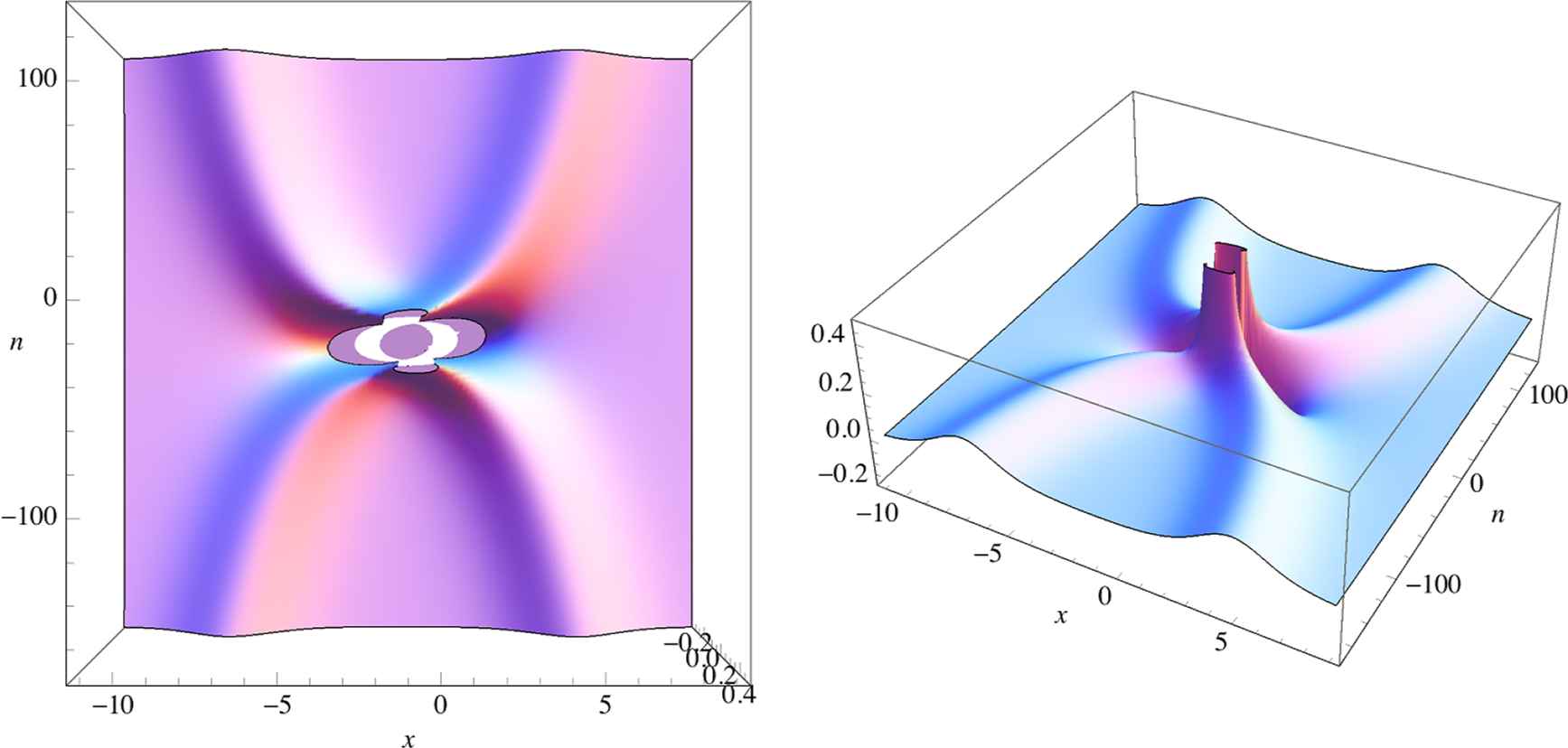
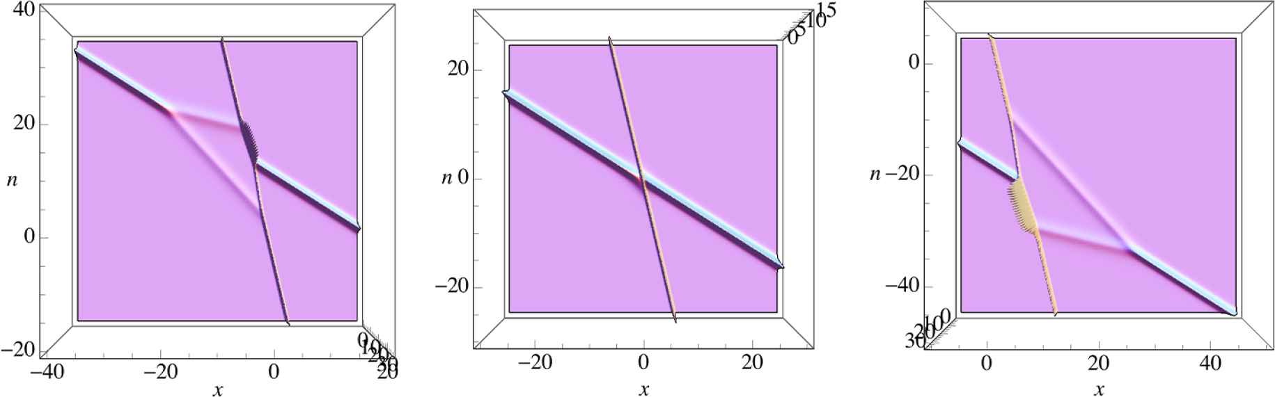
Taking A, B as Jordan blocks (hence commuting) and D = I2, we obtain solutions whose intersection with a y-slice {y = c} looks similar to the familiar 2-pole solution of the KdV: A weakly bound wave packet moving with constant velocity as n → ±∞, which consists of a regular soliton and a singular antisoliton deviating logarithmically from the common center, switching sides under collision, see Figure 6.

The plots depict the solution from Example 4.9 for y = 0, differing only in the viewpoint. Note that the white regions indicate singularities.
For A, B as before, we continue with the case that D is arbitrary. Asymptotic analysis shows that the entry in the left lower corner of D plays a privileged role, leading to solutions which are essentially different from the case D = I2. In a y-slice, such a solution is a 2-pole, but moving on steeper logarithmic curves, and not changing sides any longer. Moreover, it can be arranged that the solution is asymptotically regular. It should be mentioned that singularities occur at the place where the solitons collide, see Figure 7.
The plots depict the solution from Example 4.10 for y = 0, differing only in the viewpoint, with white regions indicating singularities.
Finally, taking A as Jordan block but B as diagonal matrix with two different entries leads to even more intriguing solutions: Here a y-slice shows two solitons moving on logarithmic paths, but these do not deviate from a common center, but each from a center of its own. Hence the solution looks as if it consists of the superposition of two 2-poles, where each of the 2-poles has lost one of its partners, see Figure 8. Splitting the asymptotic solitons into two pairs, regularity can be arranged for each of the pairs independently.
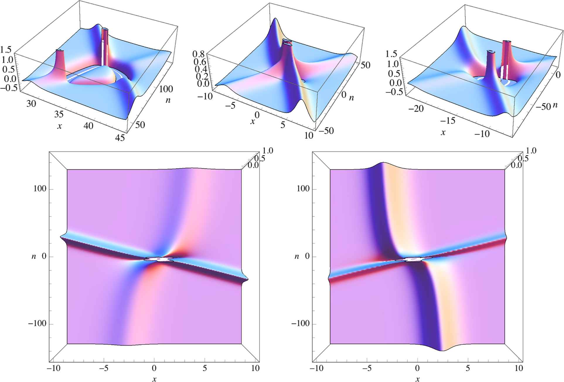
In the upper row the solution from Example 4.11 is depicted for y = −50, y = 0, and y = 20 (from left to right). The two plots in the lower row show the solution for y = 0, but in different coordinate systems, see Example 4.11 for details.
For the above mentioned three solution classes, the asymptotic analysis is given.
Similar phenomena are to be expected for the KP-II where comparable solution formulas in [32] can be exploited.
2. Solving the noncommutative two-dimensional Toda lattice
The aim of the first section is to find a general solution formula for its noncommutative (nc) version (1.4). Our result on the general operator level is the following.
Theorem 2.1.
Let E, F be Banach spaces, and A ∈ ℒ(E), B ∈ ℒ(F) invertible. Assume that the families of operators Ln = Ln(x, y) ∈ ℒ(F, E), Mn = Mn(x, y) ∈ ℒ(E, F) satisfy the following set of base equations
Theorem 2.1 generalizes [31, Theorem 2.1], where the result was obtained under the additional assumptions [A, B] = 0, which is very restrictive in applicationsb. One of our motivations was a similar generalization obtained for the noncommutative Kadomtsev-Petviashvili equations in [32].
The proof of Theorem 2.1 relies on a rather general tool box of operator identities which is presented in Appendix D.
Proof.
Let us start with some preparations. To utilize the appendix, we introduce the following operator-functions
The first three identities, which follow on applicationc of Lemma D.5, are the derivation rules
The fourth identity, which followsd from Lemma D.2 a) and Corollary D.3, allows us to handle a certain product of the operator-functions,
We are now in the position to prove Theorem 2.1. Let us begin with the left-hand side of the nc 2d-Toda lattice (1.4). Observe first that
Note that (2.4a) implies that
Hence, we find
Moreover,
Starting from this identity, and using (2.3b), (2.3c), we get for the left-hand side of the nc 2d-Toda lattice (1.4)
We next turn to the right-hand side of the nc 2d-Toda lattice (1.4). To compute the second term, we use
Analogously,
Note that (2.4b) implies that (IF + Vn)−1 = (IF + Mn+1Ln+1)−1B(IF + MnLn) B−1 = (IF + Mn+1Ln+1)−1(B + Mn+1A−1Ln+1)
Thus, for the right-hand side of the nc 2d-Toda lattice (1.4) we obtain
Comparing (2.6) with (2.10) it remains to show
3. A solution formula for the scalar 2d-Toda lattice depending on two independent operator parameters
In this section a scalarization process is introduced with which, starting from a solution of the non-commutative 2d-Toda lattice (1.4), a solution formula for the scalar lattice (1.3) can be constructed.
After introducing the necessary background from functional analysis in Subsection 3.1, we explain the main idea behind scalarization in Subsection 3.2. In Subsection 3.3, this strategy is carried out explicitely for the 2d-Toda lattice. Finally, in Subsection 3.4 we explain how the theory of elementary operators can be exploited to meet the requirements of scalarization and to simplify the solution formulas considerably.
3.1. Terminology
Before explaining our general strategy, we need some terminology. Let E, F be Banach spaces. A one-dimensional operator T ∈ ℒ(E, F) is an operator whose range is contained in a one-dimensional subspace of F. Every such operator T can be written as b ⊗ c for a vector c ∈ F and a functional b ∈ E′, where
A finite-rank operator is an operator T ∈ ℒ(E, F) with finite-dimensional range, and the space of all finite-rank operators from E into F is denoted by ℱ(E, F). We set rank(T) = dim(ran(T)). Note that
The class ℱ = ∪E,Fℱ(E, F) of finite-rank operators forms an operator ideal. Moreover, it is well-known that there is a unique trace trℱ : ∪Fℱ(F) → ℂ, which is given by
3.2. Strategy
Let us briefly explain the idea of the scalarization process. Let us assume that Vn = Vn(x, y) ∈ ℒ(F) is an operator-valued solution of the nc 2d-Toda lattice (1.4). A natural ansatz to derive a solution vn for the scalar lattice (1.3) is to apply a continuous linear functional τ to Vn, i.e. to try vn = τ(Vn). Of course the functional τ has to be chosen in a way that the solution property is maintained under its application. Since the 2d-Toda lattice is nonlinear, τ needs to be multiplicative at least in a certain sense.
To meet this requirement we introduce, for a fixed functional b ∈ F′, the subalgebra
Lemma 3.1.
For T1, T2 ∈ 𝒮b(F), it holds trℱ(T1T2) = trℱ (T1)trℱ (T2).
Proof.
We verify
This motivates the following choices:
- (1)
We assume that the operator solution Vn belongs to 𝒮b(F) for a constant, fixed b ∈ F′. In other words, Vn is one-dimensional with fixed kernel.
- (2)
For scalarization, we use the functional trℱ.
Then application of trℱ to Vn maintains the solution property.
Remark 3.3.
For a more systematic explanation of the choices (1), (2) above, we refer to [2].
For the proof of Proposion 3.2, we need two more properties for operators in 𝒮b.
Lemma 3.4.
Let T be an operator-valued function depending 𝒞1-smoothly on some variable ξ such that T(ξ) ∈ 𝒮b(F). Then also trℱ (T) depends 𝒞1-smoothly on ξ with
Proof.
By assumption, we can write T = b⊗c with a 𝒞1-smooth vector-function c : ξ → c(ξ) ∈ F. Hence
Lemma 3.5.
For T1, T2 ∈ 𝒮b(F) with IF + T1 invertible, it holds
Proof.
The assumption follows from
Proof of Propostion 3.2.
Using the tools collected above, we can directly verify that vn = trℱ (Vn) satisfies (1.3).
Note that for Step (⋆) above, linearity of trℱ, more precisely trℱ (T1 + T2) = trℱ (T1) + trℱ (T2) for T1, T2 ∈ 𝒮b(F), is used, to which end we observe that (IF +Vn)−1(Vn+1 −Vn) ∈ 𝒮b(F) for all n.
3.3. Solution formulas
Application of the scalarization technique from last subsection to the operator solution in Theorem 2.1 provides us with a first solution formula for (1.3).
Theorem 3.6.
Let E, F be Banach spaces, and A ∈ ℒ(E), B ∈ ℒ(F) invertible. Let Ln = Ln(x, y) ∈ ℒ(F, E), Mn = Mn(x, y) ∈ ℒ(E, F) be operator functions which satisfy the base equations (2.1) and the one-dimensionality condition
If (IF + MnLn) is invertible for all n ∈ and all (x, y) ∈ Ω, where Ω is an open subset of ℝ2, then
Proof.
Since Ln(x, y), Mn(x, y) satisfy the base equations (2.1), Theorem 2.1 implies that Vn = B(IF + MnLn)−1Mn(ALn − LnB−1) solves of the nc 2d-Toda lattice (1.4) on × Ω. Now the one-dimensionality condition (3.1) tells Mn(ALn − LnB−1) = b ⊗ cn with some vector function cn = cn(x, y) ∈ F, and hence
This shows Vn ∈ 𝒮b(F), and the assertion follows from Proposition 3.2.
If the operator function Ln = Ln(x, y) even takes its values in a quasi-Banach operator ideal 𝒜 which is equipped with a nice, generalized determinant, the solution formula in Theorem 3.6 can be improved considerably.
Theorem 3.7.
Let the assumptions of Theorem 3.6 be satisfied. Let, in addition, Ln = Ln(x, y) ∈ 𝒜(F, E), where 𝒜 is a quasi-Banach operator ideal admitting a continuous determinant δ. Then the solution (3.2) can be expressed as
Proof.
Let τ be the trace associated to the determinant δ by the trace-determinant theorem [24], and note this trace coincides with trℱ on ℱ(F), by uniqueness of trℱ. Hence we get
Next, using the fact that 1 + τ(T) = δ(I + T) holds for one-dimensional operators T, we obtain
3.4. Elementary operators
A natural way to satisfy the base equations (2.1) is by choosing
To this end, let 𝒜 be a quasi-Banach operator ideal, and ΦA,B : 𝒜(F, E) → 𝒜(F, E) the operator defined by
The operator ΦA,B belongs to the larger class of so-called elementary operators the structural properties of which have been extensively studied in the literature (see the survey [26] and references therein).
For the spectrum of ΦA,B the following striking formula
In particular, since we are interested in solving the Sylvester equation (3.3) with right-hand side b ⊗ c ∈ ℱ(F, E), and the finite-dimensional operators ℱ are contained in any quasi-Banach operator ideal, we are then free to choose 𝒜 arbitrarily.
Provided that 1 ∉ spec(A) · spec(B), the Sylvester equation (3.3) has the (unique) solution
A particularly convenient choice for 𝒜 is the quasi-Banach operator ideal 𝒩2/3 of 2/3-nuclear operators in the sense of Grothendieck. Recall that a bounded operator T: F → E belongs to 𝒩2/3(F, E) iff there is a representation
It was already shown by Grothendieck [12] that 𝒩2/3 is of eigenvalue-type ℓ1, i.e. operators in 𝒩2/3 possess absolutely summing eigenvalues. For quasi-Banach operator ideals of eigenvalue-type ℓ1, a deep result of White [38] states that the spectral sum trλ (i.e. the sum of the eigenvalues) is a continuous trace. By the trace extension theorem [24], this trace is unique. Using the relationship between traces and determinants on quasi-Banach operator ideals [24, Chapter 4.6], there also is a unique continuous determinant detλ on 𝒩2/3, which is spectral.
We sum up:
Proposition 3.8.
Let E, F be Banach spaces and A ∈ ℒ(E), B ∈ ℒ(F) invertible with 1 ∉ spec(A)· spec(B). Let b ∈ F′, c ∈ E, and D ∈ ℒ(E, F), and set
If detλ (IF + MnLn) ≠ 0 for all n ∈ and all (x, y) ∈ Ω, where Ω is an open subset of ℝ2, then
4. Applications
In the concluding section we discuss first applications of the solution formula in Proposition 3.8. First we re-derive line solitons [14, 16] in Subsection 4.1, then we study how resonance and web structure phenomena [4, 19] fit into the picture in Subsection 4.2. Finally, Subsection 4.3 contains some examples beyond the soliton solutions.
Usually one visualizes solutions for (1.1). Recall from the introduction that the connection between (1.3) and (1.1) is given by the dependent variable transformation wn = (1 + vn)/(1 + vn−1) − 1. One then plots the solutions for fixed values of y, the time variable, as functions of (x, n). To facilitate comparison with the literature, we start with summing up the contents of Propositions 3.8 and C.1 for (1.1).
Proposition 4.1.
Let A be an M × M-matrix, B an N × N-matrix, both invertible with 1 ∉ spec(A) · spec(B), and D an N × M-matrix. Let b ∈ ℂN, c ∈ ℂM, and let the M × N-matrix C satisfy
Note that we formulated Proposition 4.1 in the finite-dimensional setting, which is sufficient for the applications we have in mind, but it should be mentioned that there are numerous applications relying on analysis in infinite-dimensional spaces [5, 7, 8, 33].
4.1. Line solitons
Let us start with explicitly evaluating the solution formula in Proposition 4.1 for the following choices: Let M = N and let A, B are diagonal matrices, say
Furthermore let D = IN.
Given b, c ∈ ℂN, one verifies directly that the unique solution of the one-dimensionality condition ACB −C = cbt is given by
Finally, An exp(Ax − A−1y) = diag{ℓ[pj]|j}, Bn exp(−B−1x + By) = diag{1/ℓ[qj]|j}, where we have set
Then we get for the determinant (4.1) in Proposition 4.1 that
The calculation of
In particular, for N = 1 we get
Taking p1 > q1 > 0 and b1c1 > 0, to avoid singularities, we recover the 1-soliton solution (line soliton)
For fixed y, the line soliton is situated on a line in xn-space with slope d. (For visualization it is convenient to regard n as continuous variable). It is characterized by the latter and its amplitude a, where we have
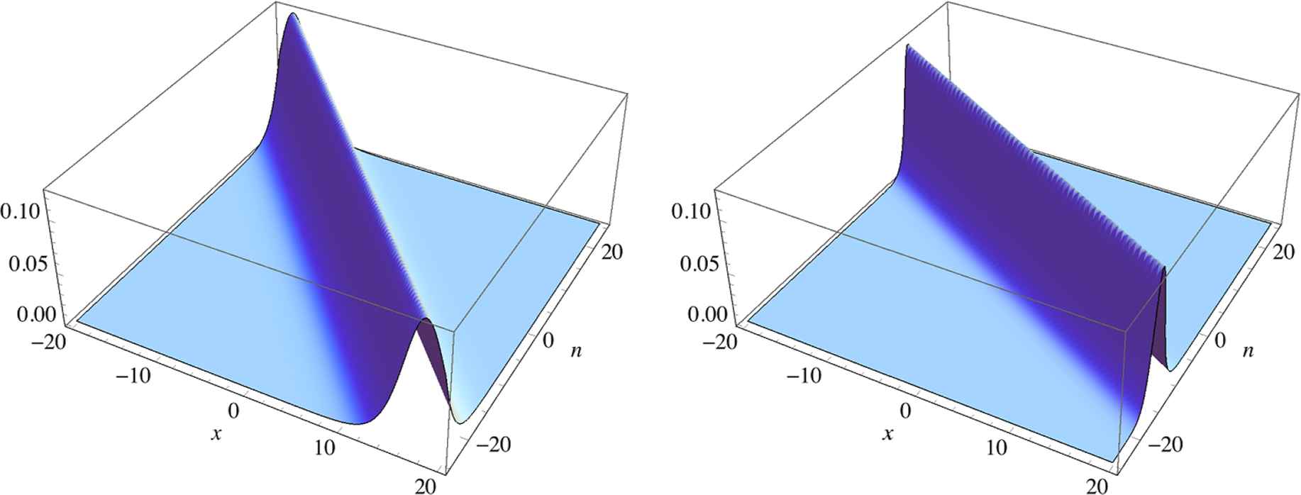
Line-solitons plotted for y = 0. The parameters in the plot to the left are (p1, q1) = (1, 0.5), in the plot to the right, (p2, q2) = (2, 1), and φ1 = φ2 = 0. Note that the solitons have the same height.
For N = 2, inspection of (4.3) shows that the solution is regular if pj > qj > 0, bjcj > 0 for j = 1, 2, and
Note that A12 encodes the position shift of the asymptotic paths of the line-solitons, which is caused by their collision.
We may assume p1 > p2 without loss of generality. Then (4.4) can be satisfied by either one of the following conditions
(O) 0 < q2 < p2 < q1 < p1,
(A) 0 < q1 < q2 < p2 < p1.
The resulting solution describes the elastic collision of two line-solitons. For condition (O), the involved solitons belong to the parameter constellations (p1, q1) and (p2, q2), constituting a collision of so-called ordinary type. For condition (A), they belong to (p1, q2) and (p2, q1), a collision of so-called asymmetric type, see [4] for details.
Example 4.2.
In Fig. 2 we provide an illustration for
Elastic collisions of two line-solitons: ordinary type (on the left) and asymmetric type (on the right), see Example 4.2 for details.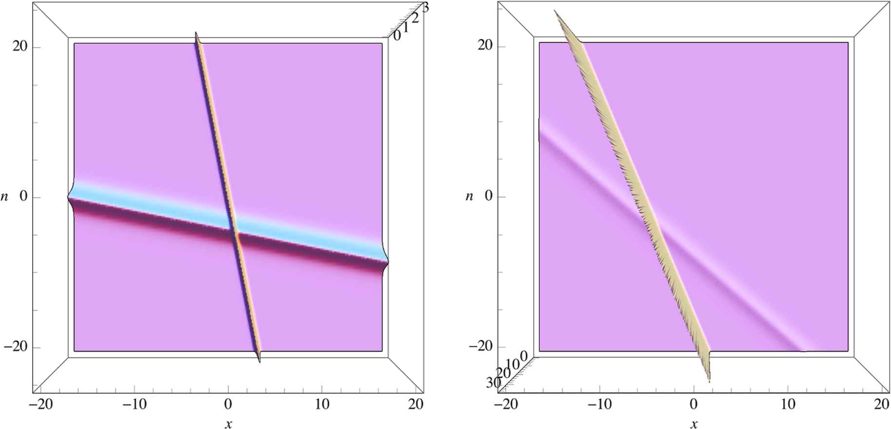
Elastic collision of two line-solitons: resonant type, plotted for y = −4, y = 0, and y = 6 (from left to right). See Example 4.5 for details.
The plot on the right corresponds to condition (O), which implies that the parameter constellation is q2 = 0.1, p2 = 0.5, q1 = 2, p1 = 15. The resulting solution shows the collision of two solitons with parameters (15, 2), (0.5, 0.1). It is plotted for y = 1.
In contrast, the plot on the left corresponds to condition (A) with the parameter constellation q1 = 0.1, q2 = 0.5, p2 = 2, p1 = 15. In this case the solution shows the collision of two solitons with parameters (15, 0.1), (2, 0.5). It is plotted for y = 10.
In [31] it is shown that the line solitons are comprised in the solution class discussed above by establishing the link to their representation in terms of Casorati determinants [14, 16].
4.2. Resonance and web structures
In [4] a solution class was studied, which not only includes elastic collision of line-solitons [15], but also soliton resonances and web structures [19]. In this subsection we first briefly recall the construction in [4]. Then we show how this class can be realized in terms of Proposition 4.1. Finally we give some examples.
The following solution class for the 2d Toda lattice (1.1) was studied in [4]:
In fact, this class contains line solitons [15] for C = C1, and fully resonant solutions [19] for C = C2, where
For this class, the following assumptions can be made:
- (1)
N < M.
- (2)
C is in reduced row echelon form (RREF) with rank(C) = N.
- (3)
The matrix C in addition satisfies that (i) each column of C contains at least one nonzero element, and (ii) each row of C contains at least one nonzero element in addition to the pivot.
Assumption (1) is no restriction since for N = M one obtains the trivial solution. Assumption (2) can be made without loss of generality. The reason is that the transformation C → C′ = GC with G ∈ GLN(ℝ) leaves the solution invariant. Note also that unless C has full rank, the determinant in (4.6) vanishes identically, and the solution is undefined. Assumption (3) serves to avoid redundancies.
Remark 4.3.
The additional assumption that
(4) all N × N-minors of C are non-negative implies regularity of the solutions (which can be easily seen by expanding the determinant).The corresponding solution class is characterised asymptotically in [4]. For the reader’s convenience, we describe in Appendix B how the asymptotics of the solution depends on the RREF of C.
The main aim of the subsection is to explain how this solution class can be realized in terms of Proposition 4.1. Note that we will not need Assumption (4). We start with the following simplification of the coefficient matrix C.
Lemma 4.4.
Without loss of generality, C = (IN D) with some N × (M − N)-matrix D. Here IN denotes the N × N-unit matrix.
Proof.
Since C is in RREF with rank(C) = N, there is a matrix Π, of size M × M, such that CΠ = (IN D) with some N × (M − N)-matrix D. Now
Inspection shows that Π−1ΘΠ corresponds to a permutation of p1,..., pM, and that Π−1K changes the Vandermonde matrix K accordingly.
Similar to the decomposition of the coefficient matrix C in an N × N-matrix and an N ×(M −N)-matrix in the above lemma, we write
To see how the corresponding solution is realized using Proposition 4.1, we set E = ℝM−N, F = ℝN, and define
By Proposition A.4, see Appendix A, the (M − N) × N-matrix
As a consequence, the solution class (4.6) is included in Proposition 4.1 with the two generating matrices A, B being diagonal, but not necessarily of the same size.
Let us illustrate the above by having a closer look at collisions of two line-solitons. Recall 0 < p1 < p2 < p3 < p4, and let θ1 = θ2 = θ3 = θ4 = 0. Elastic collision of two line-solitons correponds to the following choices for C [4, Lemma 4.1]:
(O) ordinary type:
(A) asymmetric type:
(R) resonant type:
Note that in the case (O), the second and third column of C have to be interchanged in order to bring C into the form of Lemma 4.4. Hence the following settings are needed in our formalism:
(O)
(A)
(R)
Note however, that the constants θj and the φj from our formalism not necessarily coincide.
Example 4.5.
For p4 = 15, p3 = 2, p2 = 0.5, p1 = 0.1, the elastic collision of two line-solitons of resonant type is visualized in Fig. 3 with c = 2, d = 1, compare [4, Figure 4].
Inelastic collision of two line-solitons, plotted for y = 4. Top left: type I, top right: type II, bottom left: type III, bottom right: type IV. See Example 4.6 for details.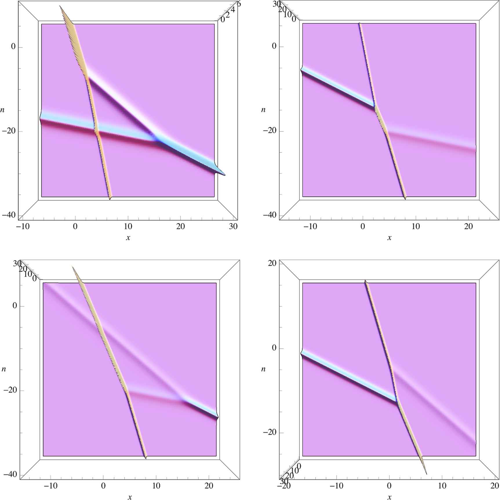
A similar transition can be made for the inelastic collision of two line-solitons. The conditions given in [4, Lemma 4.1] are:
Example 4.6.
For p4 = 15, p3 = 2, p2 = 0.5, p1 = 0.1, inelastic collision of two line-solitons is visualized in Fig. 4 with r = 1, compare [4, Figure 5].
A Miles structure, plotted for y = −4, y = 0, and y = 4 (from left to right). See Example 4.7 for details.
We conclude the present subsection with the realization of Miles structures [21]. Choosing
Note that (4.7) can be considered as the degenerated case q1 = ··· = qM = q of (4.3). In fact, starting from A = diag{p1,..., pM}, B = diag{1/q1,...,1/qM}, one arrives at the same solution class. This class has also been discussed in [31]. For fixed values of y the solutions represent tree-like structures with M line solitons for n → ∞ and 1 line soliton for n → −∞.
A similar discussion can be made for solutions generated from
Example 4.7.
The solutions in Fig. 5 correspond to the case M = 3 and the parameter constellation p1 = 0.5, p2 = 2, p3 = 15 and q = 0.1. The initial phase shifts are determined by (bcj)/(pj/q − 1) = 1.
4.3. Further examples
In this subsection we give some selected applications of Proposition 4.1 beyond the case of diagonal matrices A, B.
First we will discuss the case that A, B are 2 × 2 Jordan blocks and D = I2. Note that the corresponding solutions can be easily realized in the framework of [31], where a solution formula was established for commuting A and B, without the additional matrix parameter D. In the next case we drop the assumption D = I2. Finally we consider the case that A is a 2 × 2 Jordan block and B a 2 × 2-diagonal matrix with two different eigenvalues.
We start with the observation that the assumption that A, B are in Jordan form can be made without loss of generality.
Lemma 4.8
Let U, V be the transformation matrices of the M × M-matrix A, the N × N-matrix B into Jordan canonical form JA, JB, respectively (i.e., we have A = U−1JAU and B = V −1JBV).
Then the solution in Proposition 4.1 is not altered if we replace simultaneously A, B by JA, JB, the matrix D by VDU−1 and the vectors b, c by (V −1)tb, Uc.
Proof.
Let
First we show that replacing A, B by JA, JB and b, c by
Furthermore, by definition of the exponential function as power series, we have
By multiplicity of the determinant, p(n, x, y) = det(IN + Mn(x, y)Ln(x, y)) hence coincides with the determinant of
4.3.1. A, B (commuting) 2 × 2-Jordan blocks and D = I2
Let us now first consider the case that
Here we have introduced the ploynomials
In order to do an asymptotic investigation, we fix y and look at the solution for n → ±∞. Following the kind of arguments laid down in [29] for the one-dimensional Toda lattice, we arrive atg
This shows that, for fixed y, the solution constitutes a wave packet consisting of two partners. As a whole, the wave packet has slope d in xn-space, with the partners deviating logarithmically as n → ±∞.
Note that the asymptotics also shows that one of the partners is a (regular) soliton and the other a (singular) antisoliton. Identifying them by their regularity, one also observes that, from n → −∞ to n → ∞, the solitons cross sides. In fact, for the one-dimensional Toda lattice, which can be obtained from (1.1) by reduction [4], this kind of appearance of negaton solutions is well reflected [29].
Example 4.9.
For p = 1, q = 2, the solution discussed above is visualized in Figure 6, with b1 = 1/10, b2 = −1, c1 = 2, c2 = 1. Note that the solution is plotted in the frame (n, x − log(2)n, 0), corresponding to the fact that a line-soliton with parameters p = 1, q = 2 has slope −1/log(2) in xn-space.
4.3.2. The general case of (commuting) 2 × 2-Jordan blocks A, B
In the next case we once more consider
Inspection of the determinant in Proposition 4.1 in this case shows that in order to capture the leading terms in the asymptotic analysis it suffices to choose
Assume d3 ≠ 0 and det(D) ≠ 0. Asymptotic analysis (for fixed y) confirms that, for n → ±∞, the solution constitutes a wave packet consisting of two solitons
Observe the additional factor 2 in front of the logarithm, which is due to the fact that the polynomial appearing in the determinant p(n, x, y) is of degree 2. The even degree of the polynomial is also responsible for the fact that the solitons no longer cross sides. It is remarkable that choosing d3 and det(D) appropriately, we now can arrange that both solitons are regular.
It should be stressed that the first case (D = I2) actually is degeneration of the case above.
Example 4.10.
For p = 2 and q = 1, the solution discussed above is visualized in Figure 7, with b1 = c2 = 1 and d1 = −10, d2 = −2, d3 = −1, d4 = 1. It is plotted in the frame (n, x − log(2)n, 0).
4.3.3. Noncommuting A, B (of same size)
Finally we look at the case
Computing the determinant in Proposition 4.1 for this parameter choice, one sees that to keep the leading terms it is sufficient to choose
Assume d1, d3 ≠ 0 and det(D) ≠ 0. Recall that without loss of generality q1 > q2. For the asymptotic analysis we also fix p > q1 (note that q1 > p > q2 and q2 > p can be treated similarly). As a result, for n → ±∞ the solution consists of two solitons w(j),± (n, x, y), build with
Hence the solution consists of two different solitons, corresponding to the parameter constellations (p, q1) and (p, q2), respectively, which deviate logarithmically from their respective slopes d(1) and d(2).
Note that the collision ot the two solitons causes a phase-shift determined by A12 = (1/q1 − 1/q2)/((p/q2 − 1)(p/q1 − 1)), compare with (4.4).
Observe also that regularity of the solitons can be manipulated by the signs of d1, d3 and det(D) in the following way: One can pair the solitons arbitrarily and assign to each pair separately whether both solitons of the pair are regular or singular.
Example 4.11.
For p = 2, q1 = 1, q2 = 1/2, the corresponding solution is depicted in Figure 8 with b1 = c2 = 1 and d1 = 1, d2 = −1, d3 = −10, d4 = −1.
The two involved solitons correspond to the parameters (2, 1) and (2, 1/2). Observe that a line-soliton with parameters (2, 1) has slope −1/log2 in xn-space and one with parameters (2, 1/2) has slope −3/(4log2). The plots in the lower row of Figure 8 show the solution, plotted for y = 0, in the corresponding frames (n, x − log(2)n, 0) (left) and (n, x − 4log(2)n/3, 0) (right), the logarithmic paths of the solitons being clearly visible.
The plots in the upper row are plotted in (n, x − 7log(2)n/6, 0), where −7log(2)/6 is the arithmetic middle of −log(2) and −4log(2)/3.
A. Factorizing solutions of the Sylvester equation AX + XB = C by Vandermonde matrices
Let A = diag{α1,...,αm}, B = diag{β1,...,βn} be diagonal matrices, not necessarily of the same size, with 0 ∉ spec(A) + spec(B). Note that this spectral condition guarantees the invertibility of the elementary operator
In what follows we give a factorization of
To the data given above, we assign the m × n-Vandermonde matrix VA,n and the n × n-matrix WB as follows
Furthermore, we introduce the involution
Lemma A.1.
The following identity holds:
Proof.
By direct verification,
Hence, denoting the ij-th entry of a matrix T as usual by Tij, matrix calculation shows
As a consequence, VA,nJnWB is a solution of the Sylvester equation AX + XB = C for an appropriately chosen one-dimensional right-hand side C.
Corollary A.2.
It holds that
In summary, we have shown the following factorization result.
Theorem A.3.
Let A = diag{α1,...,αm} and B = diag{β1,...,βn} such that 0 ∉ spec(A)+spec(B). Then, for any b ∈ ℂn, c ∈ ℂm, the following factorization holds:
Proof.
From Corollary A.2 we have
The following variant of the Theorem A.3 for the elementary operator ΦA,B defined in (3.4) is used in Subsection 4.2.
Proposition A.4.
Let 0 < p1 < ··· < pM, and let A = diag{pN+1,..., pM} and B = diag{1/p1,..., 1/pN} with N < M. Furthermore, set
Then
For the proof it is useful to express the inverse of a Vandermonde matrix in the notation at hand. Note that this is a direct consequence of Lemma A.1 for n = m and B = −A.
Corollary A.5
Let the αj be pairwise different. Then
Proof of Proposition A.4.
Note first that, in the notation of this section, we have m = M − N, n = N, and KM−N = VA and KN = VB−1.By Corollary A.5,
Hence
Since B and D1 commute, it follows that
B. Classification of line solitons
For the reader’s convenience, we rehearse results from [4], where a classification of the solutions (4.6) under Assumptions (1)–(4) is given. More precisely, their asymptotic behaviour for n → ±∞ at a fixed time y is obtained in dependence of the coefficient matrix C. Note that the asymptotics is essentially independent of the particular value of y.
Recall that a single line soliton is determined by two of the parameters 0 < p1 < ··· < pM (up to a possible initial shift), and we use the abbreviation [i, j] for the soliton determined by pi < pj. Note that the pi are assumed to be generic in an appropriate sense, see [4]. Line solitons appearing asymptotically for n → −∞ are called incoming, for n → ∞ outgoing line solitons.
- 1.
There are precisely N incoming line solitons, which are characterised by
- 2.
There are precisely M − N outgoing line solitons, which are characterised by
To identify the incoming and outgoing line solitons completely, we introduce the matrices
columns no. 1,..., i − 1 and j + 1,..., M for
columns no. i + 1,..., j − 1 for
Observe that we admit empty matrices with rank 0. The following statements hold:
- 1.
If [i, j] is an incoming line soliton, then
- a)
- b)
augmenting
- a)
- 2.
If [i, j] is an outgoing line soliton, then
- a)
- b)
augmenting
- a)
For the justification of the above statements we refer to [4]. Here we confine ourselves to mentioning that the above conditions yield the asymptotic behaviour of collisions of two solitons (i.e. solutions with 2 incoming and 2 outgoing solitons) in Table 1.
| type | asymptotic line solitons | |
|---|---|---|
| n → −∞ | n → ∞ | |
| ordinary (O) | [1, 2], [3, 4] | [1, 2], [3, 4] |
| asymmetric (A) | [1, 4], [2, 3] | [2, 3], [1, 4] |
| resonant (R) | [1, 3], [2, 4] | [1, 3], [2, 4] |
| I | [1, 3], [3, 4] | [1, 2], [2, 4] |
| II | [1, 2], [2, 4] | [1, 3], [3, 4] |
| III | [1, 3], [2, 4] | [2, 3], [1, 4] |
| IV | [1, 4], [2, 3] | [1, 3], [2, 4] |
Summary of the asymptotics of (elastic and inelastic) 2-soliton solutions.
C. The two-dimensional Toda lattice in bilinear form
The aim of this appendix is to present a solution formula for the bilinear form of the 2d-Toda lattice
Our main result is
Proposition C.1.
Let E, F be a Banach spaces, A ∈ ℒ(E), B ∈ ℒ(F) invertible, and 𝒜 a quasi-Banach operator ideal admitting a continuous determinant δ. Let Ln = Ln(x, y) ∈ 𝒜(F, E), Mn = Mn(x, y) ∈ 𝒜(E, F) be operator-functions with values in 𝒜, which satisfy the base equations (2.1) and the one-dimensionality condition (3.1) with some b ∈ F′. Then
Proof.
Let τ be the trace associated to the determinant δ according to the trace-determinant theorem [24]. Recall that for a smooth operator-function ξ → T(ξ), with values in the endomorphisms on some Banach space, the following derivation rule holds [24]
We will verify that τn solves
Using the trace property τ(ST) = τ(TS) we get τ((IF + MnLn)−1B−1MnLn) = τ(MnLn(IF + MnLn)−1B−1) = τ((IF + MnLn)−1MnLnB−1), which gives
Next we turn to the right-hand side of (C.3). Using again the base equations (2.1), we find
Hence, the right-hand side of (C.3) becomes
By (3.1), we know that Vn = B(IF + MnLn)−1(b ⊗ dn) with some vector function dn, i.e. Vn = b ⊗ vn for vn = B(IF +MnLn)−1dn. In particular, also (IF + Vn)−1(Vn −Vn−1) = b ⊗ ((IF + Vn)−1(vn −vn−1)) is one-dimensional. Using that δ(I + T) = 1 + τ(T) holds for one-dimensional operators T, we conclude
Comparing (C.5) with (C.4), we see that it is sufficient to show
To this end we fall back on some identities from the proof of Theorem 2.1. together with the following identity derivedh from Appendix D,
Namely, we get
This completes the proof.
Remark C.2.
If Ω is dense in × ℝ2, Proposition C.1 yields that τn satisfies (C.1) everywhere by continuity. This will be our way to verify (C.1) in applications.
D. A toolbox of operator identities
The operator identities collected in the subsequent lemmata origin from and extend results in [30, Chapter 3]. It is worth mentioning that they also are crucial in the operator treatment of continuous integrable systems like the KP equation.
We start with some purely algebraic identities.
Lemma D.1.
Let G1, G2 be Banach spaces, and T1 ∈ ℒ(G2, G1), T2 ∈ ℒ(G1, G2) bounded linear operators such that IG1 +T1T2 (and hence also IG2 +T2T1) is invertible. Then the following identities hold
- (a)
T2(IG1 + T1T2)−1 = (IG2 + T2T1)−1T2,
- (b)
T2(IG1 + T1T2)−1T1 = IG2 − (IG2 + T2T1)−1.
Proof.
Assume that IG1 + T1T2 is invertible. Then
The same holds if one computes the product in reversed order. Hence also IG2 + T2T1 is invertible and
Note that the key in the above argument was the identity
To verify (a), we start from the analogous identity (IG2 + T2T1)T2 = T2(IG1 + T1T2) and multiply by (IG1 + T1T2)−1 from the right, and by (IG2 + T2T1)−1 from the left.
The next lemma treats products of operators of a particular form which play a key role in establishing general solution formulas for non-commutative integrable systems such as (1.4) or the nc KP equation.
Lemma D.2.
Let G1, G2 be Banach spaces, and L1 ∈ ℒ(G2, G1), L2 ∈ ℒ(G1, G2) such that IG1 + L1L2 (and hence also IG2 + L2L1) is invertible.
Let A1 ∈ ℒ(G1), A2 ∈ ℒ(G2) be invertible operators and
Define
- (a)
- (b)
Proof.
To improve readability, we write
Corollary D.3.
If
Next we turn to identities involving operator functions depending on a (scalar) variable ξ. Let us first recall the derivation rule for inverses.
Lemma D.4.
Let G be a Banach space and T be an ℒ(G)-valued function depending 𝒞1-smoothly on some variable ξ. If T(ξ) is invertible for all ξ, then T −1(ξ) is 𝒞1-smooth and
Now we look at derivation rules for operator functions with a similar structure as in Lemma D.2.
Lemma D.5.
Let G1, G2 be Banach spaces, and L1, L2 are operator-valued functions depending 𝒞1-smoothly on some variable ξ with L1(ξ) ∈ ℒ(G2, G1), L2(ξ) ∈ ℒ(G1, G2) such that IG1 +L1L2 (and hence also IG2 + L2L1) is invertible.
Let
Assume that the following base equations are satisfied
Then the following derivation rules hold:
- (a)
- (b)
Remark D.6.
Note that if
Proof.
To improve readability, we write
Observe first that, by the non-commutative product rule, and on use of the base equations, we have
Hence, by Lemma D.4,
Second, using Lemma D.1(a) for the boxed identity, we compute
Acknowledgement
The authors would like to thank the referees for careful reading and valuable remarks.
Footnotes
The 1-dimensionality condition involves two further parameters, which are less significant for the dynamic behaviour and can be neglected in this discussion.
For both (2.3a) and (2.3c), use L1(n, x, y) = Mn(x, y), L2(n, x, y) = Ln(x, y) and A1 = B, A2 = A. Then, for (2.3a) one sets
For (2.3c) on the other hand, with
Turning to (2.3b), we now use L1(n, x, y) = Ln(x, y), L2(n, x, y) = Mn(x, y), A1 = A, A2 = B, and
Then
Use again L1(n, x, y) = Mn(x, y), L2(n, x, y) = Ln(x, y) and A1 = B, A2 = A. Furthermore one sets
Recall that all functionals β on ℂN are of the form β : x ↦ btx for some b ∈ ℂN, and β ⊗ c(x) = 〈x, β 〉c = (btx)c = (cbt)x.
assuming b1c2 ≠ 0
Here we use the following notion of convergence, see [29]: For fixed x, fx(n) := f(n, x) is viewed as a mapping to the Riemann number sphere
References
Cite this article
TY  - JOUR
AU  - Tomas Nilson
AU  - Cornelia Schiebold
PY  - 2019
DA  - 2019/10/25
TI  - Solution formulas for the two-dimensional Toda lattice and particle-like solutions with unexpected asymptotic behaviour
JO  - Journal of Nonlinear Mathematical Physics
SP  - 57
EP  - 94
VL  - 27
IS  - 1
SN  - 1776-0852
UR  - https://doi.org/10.1080/14029251.2020.1683978
DO  - 10.1080/14029251.2020.1683978
ID  - Nilson2019
ER  -