Journal of Nonlinear Mathematical Physics

Volume 25, Issue 3, July 2018, Pages 462 - 484

Hopf magnetic curves in the anti-de Sitter space 𝔿13

Authors
Giovanni Calvaruso
Dipartimento di Matematica e Fisica “E. De Giorgi” Università del Salento, Prov. Lecce-Arnesano 73100 Lecce, Italy,giovanni.calvaruso@unisalento.it
Marian Ioan Munteanu
Department of Mathematics, University Alexandru Ioan Cuza of Iasi Bd. Carol I, n. 11, 700506 Iasi, Romania,marian.ioan.munteanu@gmail.com
Received 9 September 2017, Accepted 21 March 2018, Available Online 6 January 2021.
DOI
10.1080/14029251.2018.1494767How to use a DOI?
Keywords
Anti-de Sitter space; Hopf fibration; magnetic curves
Abstract

We consider the anti-de Sitter space 𝔿13 and the hyperbolic Hopf fibration h:𝔿13(1)𝔿2(1/2). Using their description in terms of paraquaternions, we study the magnetic curves of the hyperbolic Hopf vector field. A complete classification is obtained for light-like magnetic curves, showing in particular the existence of periodic examples, and emphasizing their relationship with the hyperbolic Hopf fibration. Finally, we give a new interpretation of magnetic curves in 𝔿13 using some techniques of Lie groups and Lie algebras.

Copyright
© 2018 The Authors. Published by Atlantis and Taylor & Francis
Open Access
This is an open access article distributed under the CC BY-NC 4.0 license (http://creativecommons.org/licenses/by-nc/4.0/).

1. Introduction

Let (M,g) denote an n-dimensional pseudo-Riemannian manifold and ∇ its Levi-Civita connection. A magnetic field on (M,g) is any closed two-form F on M. Through g, a magnetic field F corresponds to a skew-symmetric (1,1)-tensor field Φ, called the Lorentz force, uniquely determined by g(Φ(X),Y) = F(X,Y), for any vector fields X,Y tangent to M.

Under the action of F, a charged particle describes a trajectory γ, which satisfies the Lorentz equationγ′ γ′ = Φ(γ′). As such, magnetic curves are a natural generalization of geodesics, which satisfy the Lorentz equation in the absence of any magnetic field. However, it is a remarkable fact that magnetic curves never reduce to geodesics. In fact, given a nontrivial magnetic field F on a Riemannian manifold, there exists no affine connection whose geodesics coincide with the magnetic curves of F [5, Proposition 2.1].

A wide literature is devoted to the study of the magnetic flow and curves, also motivated by the fact that they naturally occur in several topics with an interesting physical meaning. For example, many authors pointed out that the solutions of the Lorentz force equation are Kirchhoff elastic rods. This establishes a relation between two distinct physical models, namely, the classical elastic theory and the Hall effect. The solutions of the Lorentz equation are also critical points of a certain functional (known as the Landau-Hall functional), so that magnetic trajectories are also solutions of a variational problem.

As one can expect, the first examples to be considered were the cases of magnetic curves in Riemannian surfaces and in Riemannian spaces of constant sectional curvature, successively considering cases of higher dimensions, different signatures, and less simple curvature.

A typical example of magnetic fields is obtained by multiplying the area form on a Riemannian surface (M,g) by a scalar q (usually called strength or magnitude). When (M,g) is of constant Gaussian curvature K, trajectories of such magnetic fields are well known. More precisely, on the sphere 𝕊2(r), (K=1r2), trajectories are small circles of certain radius, on the Euclidean plane they are circles, and on a hyperbolic plane 𝔿2(r), (K=1r2), trajectories can be either closed curves (when |q|>1r), or open curves. Moreover, when , or open curves. Moreover, when |q|=1r, normal trajectories are horocycles ([15,27]). This study was also extended to different ambient spaces. For example, K¨ahler magnetic fields in complex space forms were studied in [2], and explicit trajectories for K¨ahler magnetic fields in the complex projective space ℂ𝕇n were determined in [1]. If the ambient is a contact manifold, the fundamental two-form defines the so-called contact magnetic field. Interesting results are obtained when the manifold is Sasakian, namely, the angle between the velocity of a normal magnetic curve and the Reeb vector field is constant, and for their analogues of Lorentzian signature, that is, paraSasakian three-manifolds [11]. Moreover, an explicit description for normal flowlines of the contact magnetic field on a three-dimensional Sasakian manifold is known [13,14] (see also [16,21]).

In this framework, the three-dimensional case shows some special behaviors, since the Hodge star operator ⋆ and the volume form dvg of the manifold establish a one-to-one correspondence between (closed) two-forms and (divergence-free) vector fields. This leads to define the significant class of Killing magnetic fields, as the ones corresponding to Killing vector fields. It is then a natural problem to determine Killing magnetic curves of a three-dimensional pseudo-Riemannian manifold (see for example [17, 18, 25]). Such a study becomes particularly relevant when the Killing vector field defining the magnetic field has a special geometric meaning, with a special focus on light-like and periodic magnetic trajectories, the existence of closed lightlike trajectories in a Lorentzian manifold being a well known topic (see for example [8,28] and the works where they were cited). The anti-de Sitter space is a well known and relevant model in Mathematical Physics, and it has been studied under a wide range of different points of view. In this paper, we consider the anti-de Sitter space 𝔿13 and the hyperbolic Hopf fibration h:𝔿13(1)𝔿2(1/2). Although the choice of the Hopf vector field is essentially due to its geometric meaning, lying in the fact that it is tangent to the fibers of the Hopf fibration, it may be observed that principal fiber bundles often appear in Physics. Using the description of 𝔿13 and h in terms of paraquaternions, we study the magnetic curves of the hyperbolic Hopf vector field. A complete classification is obtained for its light-like magnetic curves. In particular, our study leads to show the existence of periodic examples. Moreover, we also investigate the projections of these magnetic curves on the hyperbolic plane 𝔿2(1/2). Finally, the Lie group structure of the anti-de Sitter space also permits another interpretation of the magnetic curves corresponding to the (Killing, right invariant) hyperbolic vector field and illustrates their link with invariant geodesics.

The paper is organized in the following way. In Section 2 we report some basic facts about magnetic curves and the description of 𝔿13 in terms of paraquaternions. Then, in Section 3 we obtain a complete classification of light-like magnetic curves of the hyperbolic Hopf vector field. In particular, we prove the existence of periodic light-like Hopf magnetic curves on 𝔿13, quantized in the set of rational numbers. In Section 4 we show that projections in 𝔿2(1/2) of Hopf light-like magnetic curves via the hyperbolic Hopf fibration, have constant curvature. In Section 5 we investigate the geometry of light-like magnetic curves in the hyperbolic Hopf tubes of their projections in 𝔿2(1/2). Finally, in Section 6 we give a new interpretation of magnetic curves in 𝔿13 using some techniques of Lie groups and Lie algebras.

2. Preliminaries

2.1. Magnetic curves

A magnetic curve represents the trajectory of a charged particle moving on the manifold under the action of a magnetic field. A magnetic field on an n-dimensional Riemannian manifold (M,g), is a closed two-form F. The corresponding Lorentz force of the magnetic field F is the skew-symmetric (1,1)-tensor field Φ defined by

gΦ(X),Y)=F(X,Y),X,Yχ(M).

The magnetic trajectories of F are curves γ on M that satisfy the Lorentz equation

γγ=Φ(γ).(2.1)

The curve γ is also known as the flowline of the dynamical system associated with the magnetic field F. See e.g. [5]. Obviously, magnetic curves naturally generalize geodesics. More precisely, the equation satisfied by the geodesics of M, namely

γγ=0
is nothing but the Lorentz equation in the absence of any magnetic field. Therefore, from the point of view of dynamical systems, a geodesic corresponds to a trajectory of a particle when F = 0. An important property of magnetic curves is that their speed v(t) is a constant v0 and hence, their kinetic energy is also constant. This is a straightforward consequence of the skew-symmetry of the Lorentz force. When the magnetic curve γ(t) is arc length parametrized (v0 = 1), it is called a normal magnetic curve.

In the case of a three-dimensional (pseudo-) Riemannian manifold (M,g), two-forms and vector fields may be identified via the Hodge star operator ⋆ and the volume form dvg of the manifold. Thus, magnetic fields and divergence-free vector fields are in one-to-one correspondence (see for example [14]). In particular, Killing vector fields define an important class of magnetic fields, called Killing magnetic fields. Recall that a vector field V on M is Killing if and only if it satisfies the Killing equation:

g(YV,Z)+g(ZV,Y)=0
for every vector fields Y,Z on M, where ∇ is the Levi-Civita connection on M.

On a three-dimensional pseudo-Riemannian manifold (M,g), one can define the cross product of two vector fields X,Yχ(M) as

g(X×Y,Z)=dvg(X,Y,Z),Zχ(M).

If V is a Killing vector field on M, let FV = ıV dvg be the corresponding Killing magnetic field, where ı denotes the interior product. Then, the Lorentz force of FV is given by (see [14])

Φ(X)=V×X.

Consequently, the Lorentz force equation (2.1) can be rewritten as

γγ=V×γ.

2.2. The hyperbolic Hopf fibration

We shall now present the hyperbolic counterpart of the Hopf fibration 𝕊3 → 𝕊2(1/2). For further details, we may also refer to [10] and [12].

Let us consider 24, the four-dimensional pseudo-Euclidean space equipped with the pseudo-Riemannian flat metric

,=dx02dx12+dx22+dx32
of neutral signature (2,2). The anti-de Sitter (three-)space 𝔿13 is the hypersurface of 24, defined by [19,26]
{x=(x0,x1,x2,x3)4:x02x12+x22+x32=1}.

In terms of complex coordinates z = x0 + ix1, w = x2 + ix3, consider ℂ2 endowed with the pseudo-scalar product q1,q2=e(z1z¯2+w1w¯2), where qa = (za,wa), a = 1,2 and denote it by 12. Then, the above description of 𝔿13 becomes

𝔿13={(z,w)12:|z|2+|w|2=1}.

Similarly, the pseudo (three-)sphere is given by

𝕊23={x=(x0,x1,x2,x3)24:x02x12+x22+x32=1}={(z,w)2:|z|2+|w|2=1}.

Equipping both 𝔿13 and 𝕊23 with the Lorentzian metrics induced from 〈, 〉 as hypersurfaces of 24, they are complete Lorentzian manifolds, of constant sectional curvature −1 and 1 respectively. Moreover, 𝔿13 and 𝕊23 are both diffeomorphic to 𝕊1×ℝ2, and the map σ:2424, σ(x0, x1, x2, x3) = (x2, x3, x0, x1) is an anti-isometry which carries 𝔿13 onto 𝕊23 and conversely.

We now consider the canonical projection π : ℂ2 −{0} → ℂ𝕇1 which defines the complex projective line ℂ𝕇1. When we restrict π to 𝔿132{0}, we obtain a diffeomorphism from 𝔿13 onto the unit disk B2 = {ζ ∈ ℂ : |ζ| < 1}, explicitly described by ζ = π(z,w) = w/z.

Next, we consider the (Riemannian) hyperbolic two-space, as the surface 𝔿2(r)13, of constant curvature −1/r2 < 0 with r > 0 given by

𝔿2(r)={y=(y1,y2,y3)13:y12+y22y32=r2andy3>0}.

Let p denote the stereographic projection p from the point (0,0, −1), that is,

p:𝔿2(1)B2
(y1,y2,y3)ζ=(y11+y3,y21+y3)
and the homothety ηr : 𝔿2(1) → 𝔿2(r), y ry. Then, the hyperbolic Hopf map h is explicitly given by
h=η12p1π:𝔿13(1)𝔿2(1/2)(z,w)(z¯w,|z|2+|w|22)×.

Similarly to the Riemannian case, h is a submersion with geodesic fibres, which can be defined as the orbits of the 𝕊1-action

𝕊1×𝔿13𝔿13(eit,(z,w))(eitz,eitw).

In particular, for any x=(x0,x1,x2,x3)𝔿13, the vector field

ξx=(x1,x0,x3,x2)
is tangent to the fibres of the hyperbolic Hopf map and 〈ξx,ξx〉 = 〈x,x〉 = −1. For this reason, in analogy with the Riemannian case, we call ξ the hyperbolic Hopf vector field. It is easily seen that ξ is a globally defined Killing vector field [12].

We shall now describe the anti-de Sitter space 𝔿13 in terms of paraquaternions, referring to [12] for more details (see also [22]). Consider the algebra 𝔹 of paraquaternionic numbers over ℝ generated by {1,i, j,k}, where −i2 = j2 = 1 and k = i j = − ji (they are also known as Gödel quaternions or split quaternions in Theoretical Physics). This is an associative, noncommutative and unitary algebra over ℝ. The conjugate of a paraquaternonic number x = x0 + x1i + x2 j + x3k, is given by x¯=x0x1ix2jx3k, and the norm of x is given by

x2=xx¯=x02+x12x22x32.

Obviously, the norm of a paraquaternion corresponds to the pseudo-Euclidean metric 〈, 〉 on 24, namely

x,x=xx¯.

It is easy to check that the paraquaternionic multiplication can be expressed in terms of complex numbers as

(z1,w1)(z2,w2)=(z1z2+w1w¯2,z1w2+w1z¯2).

Therefore, in terms of paraquaternions, the anti-de Sitter three-space 𝔿13(1) corresponds to

𝔿13={x𝔹:xx¯=1}.

Note that 1𝔿13 and the multiplicative structure on 𝔹 induces a group structure on 𝔿13. Moreover, the vectors {i, j,k} form a pseudo-orthonormal basis of T1𝔿13, the tangent space at 1 to 𝔿13, with 〈i,i〉 = −1, 〈 j, j〉 = 〈k,k〉 = 1.

In terms of paraquaternions, the hyperbolic Hopf vector field at x ∈ 𝔹 is given by

ξx=ix.

So, if we put

Ux=jx,Vx=kx,
for any x ∈ 𝔹, then ,U,V} is a global pseudo-orthonormal frame field on 𝔿13. Let g be the metric induced on 𝔿13 by 〈, 〉. With respect to g, the vector field ξ is time-like, while U,V are space-like. If ∇ is the Levi-Civita connection of the metric g, we have (see also Section 4 in [12])
ξξ=0,Uξ=V,Vξ=U,ξU=V,UU=0,VU=ξ,ξV=U,UV=ξ,VV=0.(2.2)

On 𝔿13 we can consider the usual cross product, defined by g(X ×Y,Z) = dvg(X,Y,Z) for all X,Y,Z tangent to 𝔿13. Here, by dvg we denote the volume form on 𝔿13, defined by the Lorentzian metric g. Subsequently, we have

ξ×U=V,U×V=ξ,V×ξ=U.

3. Hopf magnetic curves of 𝔿13

Consider a smooth curve γ=γ(s)=(x0(s),x1(s),x2(s),x3(s))𝔿13. Since ξ is Killing, we define a magnetic curve γ, corresponding to ξ, as a solution of the equation

γ˙γ˙=qξ×γ˙,(3.1)
where q ≠ 0 is the strength (see also [14,17,18,25]). We call γ a Hopf magnetic curve on 𝔿13. Since {ξ,U,V} is a frame on 𝔿13, there exist some smooth functions T1,T2,T3 (depending on s), such that the velocity γ˙=T1ξ+T2U+T3V. Moreover, T1 is a real constant. Indeed, using (2.2) and (3.1) we have
T˙1=ddsg(γ˙,ξ)=g(qξ×γ˙,ξ)+g(γ˙,γ˙ξ)=0.

Note that g(γ˙,γ˙) is constant. Therefore, the causal character of γ is the same at each point and hence, it depends on the initial value of γ˙. From now on, we focus on the case when γ is a light-like magnetic curve of ξ.

Remark that γ is light-like if and only if 0=γ˙2=T12+T22+T32. In this case, T1 ≠ 0, otherwise γ reduces to a point.

Using (2.2), we can compute γ˙γ˙. By a standard calculation, we get

γ˙γ˙=T˙1ξ+T˙2U+T˙3V.

On the other hand, from (3.1) we have

γ˙γ˙=qξ×γ˙=q(T3U+T2V).

Comparing the two above equations for γ˙γ˙, we get (again) T˙1=0 and

{T˙2=qT3,T˙3=qT2.(3.2)

Integrating the above system of ordinary differential equations, we obtain the general solution as

T2(s)=iT3(s)=αeiqs,
with α ∈ ℂ. Then, T12=|α|2. Moreover, after a suitable translation in parameter s, one can make s real and sgn(α) = sgn(T1), giving also α = T1.

Next, since ξγ(s) = i · γ(s), Uγ(s) = j · γ(s) and Vγ(s) = k · γ(s), we have

γ˙(s)=(T1(s)i+T2(s)j+T3(s)k)γ(s).

Therefore, as γ(s) = x0(s)+x1(s)i+x2(s)j +x3(s)k, the components x0(s),...,x3(s) of γ satisfy the following system of differential equations

(x˙0x˙1x˙2x˙3)=(0T1T2T3T10T3T2T2T30T1T3T2T10)(x0x1x2x3).

In terms of complex coordinates, γ(s) = (z(s),w(s)), the above system becomes

{z˙=T1iz+(T2+iT3)w¯,w˙=T1iw+(T2+iT3)z¯.(3.3)

Thus, to solve (3.3), we introduce the new complex functions

ρ:=eiT1sz,φ:=eiT1sw,(3.4)
so that (3.3) becomes
{ρ˙=αei(q2T1)sφ¯,φ˙=αei(q2T1)sρ¯.(3.5)

Taking the derivative with respect to s in both equations in (3.5) and replacing ρ˙, φ˙ again from (3.5), we get the second order complex differential equations

ρ¨i(q2T1)ρ˙T12ρ=0,φ¨i(q2T1)φ˙T12φ=0.(3.6)

So, the above equations are both of the form

f¨iaf˙T12f=0,(3.7)
where a = q − 2T1. Putting f=eias2, from (3.7) we get the standard equation
θ¨(T12a24)θ=0,
whose solution depends on the sign of T12a24=q(T1q4). We shall now treat separately the three cases determined by the possible values of q(T1q4).

First Case: q(T1q4)=0.

Then, T1=q4, as q ≠ 0. Going back to equations (3.6), we get

ρ=eiqs4(a1s+a2),φ=eiqs4(b1s+b2),
for some complex constants a1,a2,b1,b2. By a standard calculation, from (3.5) we obtain
b1=ia¯1,b2=4a¯1qia¯2.(3.8)

Thus, replacing into (3.4), we find

γ=(z(s),w(s))=eiqs2(a1s+a2,4a¯1qi(a¯1s+a¯2)).

It is easy to check that γ𝔿13 implies 16|a1|2q28qm(a¯1a2)+1=0.

We can now rewrite γ𝔿1324 as follows:

γ(s)=(cos(qs2)+isin(qs2))(sV1+V2),
where, if a1 = α1 + 2,a2 = β1 + 2,b1 = λ1 + 2,b2 = μ1 + 2, we put
V1(α1,α2,λ1,λ2),V2=(β1,β2,μ1,μ2).

Since γ is a light-like curve on 𝔿13 then, with respect to 〈, 〉, the vector field V1 is light-like and V2 is a unitary and time-like vector field. Moreover, they are orthogonal and satisfy

V1,iV2=q4.

Applying an isometry (that is, a pseudo-orthogonal transformation) of the ambient space, without loss of generality we may take V2 = (1,0,0,0). Then, by (3.8) we immediately conclude that V1=(0,q4,q4,0), which gives

γ(s)=(cos(qs2)+qs4sin(qs2),sin(qs2)qs4cos(qs2),qs4cos(qs2),qs4sin(qs2)).(3.9)

This curve cannot be periodic. Contrary, supposing that γ(0) = γ(P) for a certain P > 0, and comparing the third and the fourth components respectively, we obtain the contradiction qPcos(qP2)=qPsin(qP2)=0. Finally, the curve γ is a helix. See the Appendix A . Summarizing, we proved the following result.

Theorem 3.1.

Let γ𝔿13 denote a light-like magnetic curve of the hyperbolic Hopf vector field ξ, that is, a solution of γ˙γ˙=qξ×γ˙, with q ≠ 0. If g(γ˙,ξ)=q4, then γ is a light-like helix, explicitly described, up to pseudo-orthogonal transformations, by equation (3.9). These light-like magnetic curves are never periodic.

Second Case: q(T1q4)=ω2, ω > 0.

In this case,

ρ=ei(q2T1)s(a1cosh(ωs)+a2sinh(ωs)),φ=ei(q2T1)s(b1cosh(ωs)+b2sinh(ωs)),
for some complex constants a1,a2,b1,b2, where b1,b2 can be explicitly determined in terms of a1,a2 by means of (3.5). Replacing into (3.4), we obtain
γ=(z(s),w(s))=eiqs2(a1cosh(ωs)+a2sinh(ωs),b1cosh(ωs)+b2sinh(ωs)).

Setting a1 = α1 + 2, a2 = β1 + 2, b1 = λ1 + 2, b2 = μ1 + 2, we get

γ(s)=(cos(qs2)+isin(qs2))(α1cosh(ωs)+β1sinh(ωs)+i(α2cosh(ωs)+β2sinh(ωs),λ1cosh(ωs)+μ1sinh(ωs)+i(λ2cosh(ωs)+μ2sinh(ωs))).

Since γ𝔿13, we have 〈γ(s),γ(s)〉 = −1, which yields, by the above description of γ,

{α12α22+λ12+λ22=1,β12β22+μ12+μ22=1,α1β1α2β2+λ1μ1+λ2μ2=0.

Considering the following vector fields in 24

V1=(α1,α2,λ1,λ2),V2=(β1,β2,μ1,μ2),
we obtain that V1 (time-like) and V2 (space-like) are unitary and orthogonal. Then
γ(s)=(cos(qs2)+isin(qs2))(cosh(ωs)V1+sinh(ωs)V2).

Without loss of generality, applying an isometry in the ambient space, it is enough to consider

V1=(cosh(ψ),0,sinh(ψ),0),V2=(0,sinh(ϑ),0,cosh(ϑ)).

Thus,

γ(s)=(cosh(ψ)cosh(ωs)cos(qs2)sinh(ϑ)sinh(ωs)sin(qs2),cosh(ψ)cosh(ωs)sin(qs2)+sinh(ϑ)sinh(ωs)cos(qs2),sinh(ψ)cosh(ωs)cos(qs2)cosh(ϑ)sinh(ωs)sin(qs2),sinh(ψ)cosh(ωs)sin(qs2)+cosh(ϑ)sinh(ωs)cos(qs2)).(3.10)

This curve is a helix. See the Appendix A . Moreover, by an argument similar to the one applied for the first case, we conclude that the curve given by (3.10) is not periodic.

Thus, we proved the following.

Theorem 3.2.

Let γ𝔿13 denote a light-like magnetic curve of the hyperbolic Hopf vector field ξ, that is, a solution of γ˙γ˙=qξ×γ, with q ≠ 0. If g(γ˙,ξ)=T1 and q(T1q4)=ω2, ω > 0, then γ is a light-like helix, explicitly described, up to pseudo-orthogonal transformations, by (3.10). These light-like magnetic curves are never periodic.

Third Case: q(T1q4)=ω2, ω > 0.

We now have

ρ=ei(q2T1)s(a1cos(ωs)+a2sin(ωs)),φ=ei(q2T1)s(b1cos(ωs)+b2sin(ωs)),
for some complex constants a1,a2,b1,b2, with b1,b2 determined in function of a1,a2 using (3.5). Then, (3.4) yields
γ=(z(s),w(s))=eiqs2(a1cos(ωs)+a2sin(ωs),b1cos(ωs)+b2sin(ωs)).

We set again, as in the previous cases, a1 = α1 + 2, a2 = β1 + 2, b1 = λ1 + 2, b2 = μ1 + 2 and we find

γ(s)=(cos(qs2)+isin(qs2))(α1cos(ωs)+β1sin(ωs)+i(α2cos(ωs)+β2sin(ωs),λ1cos(ωs)+μ1sin(ωs)+i(λ2cos(ωs)+μ2sin(ωs))).

Since 〈γ(s),γ(s)〉 = −1, we immediately obtain

{α12α22+λ12+λ22=1,β12β22+μ12+μ22=1,α1β1α2β2+λ1μ1+λ2μ2=0.

Consider V1 = (α1,α2,λ1,λ2) and V2 = (β1,β2, μ1, μ2), two constant vectors in 24, which are unitary, time-like and 〈V1,V2〉 = 0.

We can now describe γ as follows:

γ(s)=(cos(qs2)+isin(qs2))(cosh(ωs)V1+sinh(ωs)V2).

Up to an isometry of the ambient space, it suffices to take

V1=(cosh(ψ),0,sinh(ψ),0),V2=(0,εcosh(ϑ),0,sinh(ϑ))
for some real constants ψ and ϑ, where ε = sgn(q).

Thus,

γ(s)=(cosh(ψ)cos(ωs)cos(qs2)+εcosh(ϑ)sin(ωs)sin(qs2),cosh(ψ)cos(ωs)sin(qs2)εcosh(ϑ)sin(ωs)cos(qs2),sinh(ψ)cos(ωs)cos(qs2)sinh(ϑ)sin(ωs)sin(qs2),sinh(ψ)cos(ωs)sin(qs2)+cos(ϑ)sin(ωs)cos(qs2)).(3.11)

We have the following result.

Theorem 3.3.

Let γ𝔿13 denote a light-like magnetic curve of the hyperbolic Hopf vector field ξ, that is, a solution of γ˙γ˙=qξ×γ, with q ≠ 0. If gγ˙,ξ=T1 and q(T1q4)=ω2, with ω > 0, then γ is a light-like helix, explicitly described, up to pseudo-orthogonal transformations, by (3.11). If ψ + εϑ ≠ 0, then these light-like magnetic curves are periodic if and only if

qω𝕈.

Proof.

The fact that γ is a helix is proved in the Appendix A . For the second part of the statement, suppose that γ(s) = γ(s + P), for all s and some P > 0. The curve γ has the following general form

γ(s)=(acos(λs)+bcos(μs),asin(λs)bsin(μs),ccos(λs)+dcos(μs),csin(λs)dsin(μs)),
where a,b,c,d are real constants and λ, μ are non-zero real constants with λμ. In our case λ=ω+q2, μ=ωq2 and
a=12(cosh(ψ)εcosh(ϑ)),b=12(cosh(ψ)+εcosh(ϑ)),
c=12(sinh(ψ)+sinh(ϑ)),d=12(sinh(ψ)sinh(ϑ)).

In the case when adbc ≠ 0 we know that γ is periodic if and only if λμ𝕈. Moreover, adbc = 0 is equivalent to sinh(ψ + εϑ) = 0. Henceforth, if ψ + εϑ ≠ 0, the curve γ is periodic if and only if qω is a rational number.

Remark 3.1.

If ψ + εϑ = 0, the curves γ given in (3.11) have the form

γ(s)=(cosh(ψ)cos(λs),cosh(ψ)sin(λs),sinh(ψ)cos(λs),sinh(ψ)sin(λs)),
where λ = q/2 − εω. Hence, they are always periodic.

Remark 3.2.

The existence of closed trajectories is a fascinating topic in dynamical systems. In [14], periodic orbits of the contact magnetic field on the unit three-sphere were found and a condition for periodicity was obtained. These results were generalized in [21] to Berger spheres of dimension three. In Physics, such a condition for periodicity is known as a quantization principle. In Theorem 3.3. our criterion of periodicity q/ω ∈ 𝕈 states that the set of periodic light-like magnetic curves on 𝔿13 of the hyperbolic Hopf vector field ξ of the third type are quantized in the set of rational numbers.

4. Projections in 𝔿2 of Hopf magnetic curves

As we have already reported in Section 2, the hyperbolic Hopf map is defined by

h:𝔿13(1)𝔿2(1/2),(z,w)(z¯w,|z|2+|w|22)×13.

Denoting by g¯ the usual Riemannian metric on 𝔿2(1/2), the map h becomes a pseudo-Riemannian submersion. We now investigate the geometry of the curve γ¯=hγ, that is, the projection of a light-like Hopf magnetic curve γ𝔿13 via the hyperbolic Hopf map. Let γ be a light-like magnetic curve in 𝔿13(1), given by γ(s) = (z(s),w(s)), where the complex functions z and w satisfy (3.3). We first prove the following result.

Theorem 4.1.

The projection γ¯ of a light-like Hopf magnetic curve γ𝔿13(1) via the hyperbolic Hopf map is a curve of constant curvature in 𝔿2(1/2).

Proof.

We compute the curvature κ¯ of γ¯ and show that it is a constant. We first compute γ¯˙. Using (3.3) and (3.2), we get

γ¯˙=((T2iT3)w2+(T2+iT3)z¯2,2e((T2iT3)zw)).

In particular, g¯(γ¯˙,γ¯˙)=(T22+T32)(|z|2|w|2)2=T12. Therefore, s¯=T1s is the arc-length parameter for γ¯, and the unit tangent of γ¯ is T¯=1T1γ¯˙. We also find

γ¯¨=((2T1q)i[(T2iT3)w2(T2+iT3)z¯2]+4T12z¯w¯,2T12(|z|2+|w|2+2(2T1q)e(i(T2iT3)zw)).

If ¯ denotes the Levi-Civita connection of g¯, then the curvature of γ¯ is given by

¯T¯T¯=κ¯N¯,
where N¯ is the unit normal of γ¯. A classical computation yields
κ¯N¯=1T12γ¯¨4γ¯.

Therefore, we may write

κ¯N¯=2T1qT12(i[(T2iT3)w2(T2+iT3)z¯2],2e(i(T2iT3)zw)).

Consequently, κ¯=|2T1qT1| is a constant.

Remark 4.1.

Recall the following fact about curves of constant curvature in the hyperbolic plane 𝔿2(r) (r > 0) of curvature −1/r2. Let γ¯ be such a curve and κ¯ be its geodesic curvature; then γ¯ belongs to the following list:

  • if κ¯(0,r), then the curve γ¯ is contained in an equidistant curve from a geodesic;

  • if κ¯=r , then γ¯ is part of a horocycle;

  • if κ¯>r, then the curve γ¯ is contained in a circle.

Remark 4.2.

This classification, together with the above Theorem 4.1. completely describes the projections of light-like Hopf magnetic curves in the hyperbolic plane.

We shall now explicitly describe all three cases discussed in the previous Section, also providing some examples corresponding to each of them.

For the (Riemannian) hyperbolic plane 𝔿2(1/2), we consider the hyperboloid model, namely, 𝔿2(1/2)={y=(y1,y2,y3)13:y12+y22y32=14}.

In the first case, the magnetic curve γ is given by (3.9). Its projection via the Hopf map is then parametrized by

γ¯(s)=(qs4,q2s216,12+q2s216).

This represents the intersection of the hyperbolic plane (as upper sheet of the hyperboloid) with the light-like plane with equation {y3y2=12}. A particular example is illustrated in the following Figure 1.

Fig. 1.

Projection of a light-like magnetic curve (3.9) on 𝔿2(1/2)

In the second case, the magnetic curve γ is given by (3.10), and the projection is given by

γ¯(s)=12(sinh(ψϑ)cosh(ψ+ϑ)+cosh(ψϑ)sinh(ψ+ϑ)cosh(2ωs),cosh(ψϑ)sinh(2ωs),sinh(ψϑ)sinh(ψ+ϑ)+cosh(ψϑ)cosh(ψ+ϑ)cosh(2ωs)).

It is not difficult to check that γ¯ is now the intersection of the hyperbolic plane with the time-like plane {y1cosh(ψ+ϑ)y3sinh(ψ+ϑ)=12sinh(ψϑ)}. Particular examples are shown in the following Figure 2.

Fig. 2.

Projection of a light-like magnetic curve (3.10) on 𝔿2(1/2): (left) ψ=ϑ=12, ω=12; (right) ψ=1, ϑ=0, ω=12e

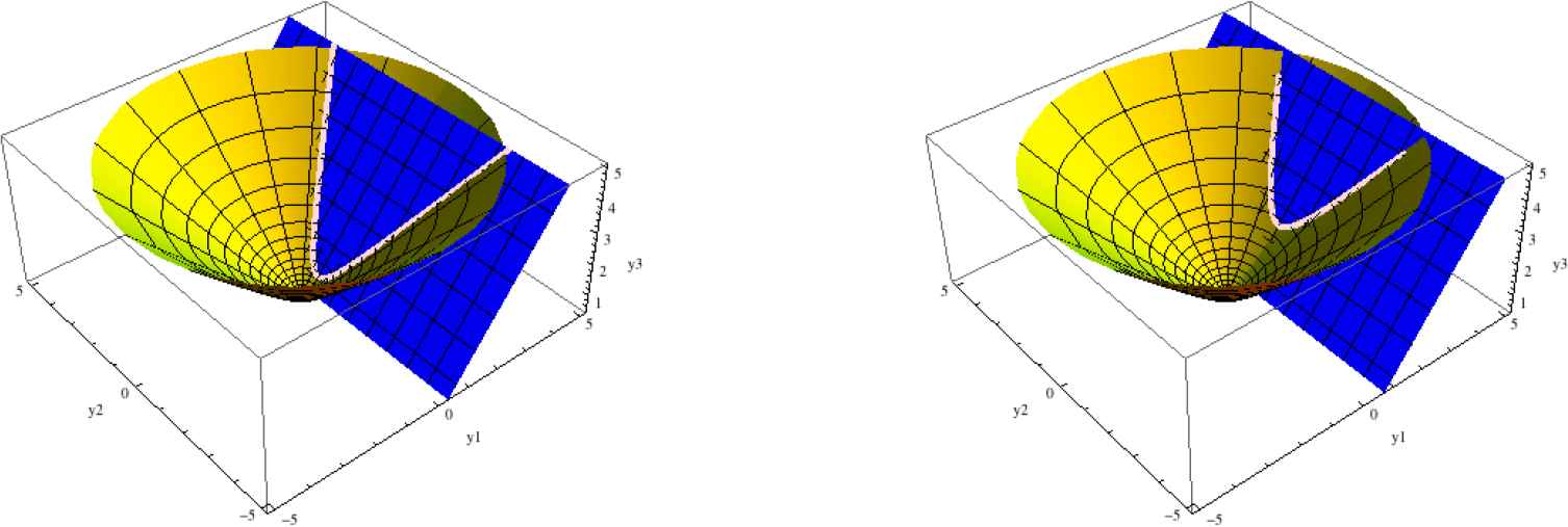
Finally, the magnetic curve given by (3.11) projects onto the curve γ¯ on 𝔿2(1/2) parametrized by

γ¯(s)=12(sinh(ψεϑ)cosh(ψ+εϑ)+sinh(ψ+εϑ)cosh(ψεϑ)cos(2ωs),εsinh(ψ+εϑ)sin(2ωs),cosh(ψϑ)cosh(ψ+ϑ)+sinh(ψϑ)sinh(ψ+ϑ)cos(2ωs)),
which lies at the intersection of the hyperbolic plane with the space-like plane
{y1sinh(ψεϑ)y3cosh(ψεϑ)=12cosh(ψ+εϑ)}.

See the following Figure 3 for particular examples. We may remark that in this case, the projection γ¯ is a closed curve on 𝔿2(1/2).

Fig. 3.

Projection of a light-like magnetic curve (3.11) on 𝔿2(1/2): (left) ψ= ϑ=1, ω=12e2; (right) ψ=32, ϑ = 0, ω=12e32

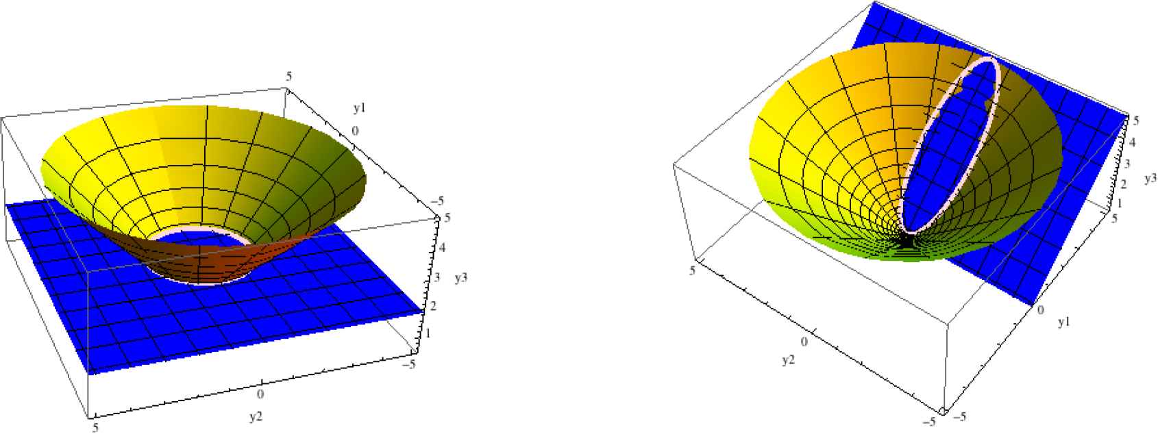
5. Light-like magnetic curves on the hyperbolic Hopf tube

Let β : I ⊂ ℝ → 𝔿2(1/2), 0 ∈ I, be a curve on 𝔿2(1/2) (not necessarily parametrized by arc-length). For any (z0,w0)𝔿13 such that h(z0,w0) = β(0), there exists a unique curve β^, known as the horizontal lift of β, such that β^(0)=(z0,w0), β^ is orthogonal to ξ and β^ projects to β, i.e. h(β^(s))=β(s), for any sI.

We then call hyperbolic Hopf tube over β its complete lift to 𝔿13, given by

Hβ:=h1(β)={eitβ^(s):t,sI}.

Consider now the following parametrization of Hβ :

F:I×𝔿13(s,t)eitβ^(s).

The tangent plane to the surface Hβ is spanned by Fs and Ft, which are computed as

{Fs(s,t)=eitβ^(s),Ft(s,t)=iF(s,t)=ξF(s,t).

When β is the projection of a magnetic curve on 𝔿13, it has constant speed v (not necessarily equal to 1). We have

h*,β^(s)β^(s)=β(s),sI.

On Hβ we consider the induced metric from the metric 〈, 〉 of 𝔿13. We also have that ,=h*g¯ , where g¯ is the metric on the hyperbolic plane 𝔿2(1/2). Consequently, we can compute the induced metric gβ on Hβ and we obtain

gβ=v2ds2dt2,
which yields at once the following result.

Proposition 5.1.

The hyperbolic Hopf tube Hβ over a constant speed curve β is flat.

The unit normal at β^(s) to Hβ is the horizontal lift at β^(s) of the unit normal ν(s) at β(s), denoted by ν^(s). Hence, β^(s) is a horizontal vector orthogonal to β^(s). The unit normal at F(s,t) to Hβ is then given by N(s,t)=eitν^(s).

An arbitrary curve Γ on Hβ writes (locally) as t = t(s) and so, it may be expressed as Γ(s)=eit(s)β^(s). It follows that

Γ(s)=t(s)ξΓ(s)+eit(s)β^(s).

Let now γ be a magnetic curve on 𝔿13, parametrized by pseudo-arc length s. Denoting by β its projection on 𝔿2(1/2), we obviously have γHβ .

As we have seen above, γ˙ has a component along ξ and a horizontal component. From the previous Sections we know that γ˙(s),ξγ(s) is a constant c. We now prove the following.

Theorem 5.1.

A light-like magnetic curve γ on 𝔿13 is a geodesic on the corresponding hyperbolic Hopf tube.

Proof.

From the Lorentz equation (3.1) we conclude that γ˙γ˙, being orthogonal to ξ and γ˙, is orthogonal to Hβ . Using the Gauss’s formula, we then obtain at once that γ is a geodesic on Hβ .

Remark 5.1.

We may express the equation of γ in terms of coordinates on Hβ . More precisely, since γHβ, parametrize γ as t = t(s). Then γ˙=t(s)ξy(s)+eit(s)β^(s). It follows that

c=γ˙,ξγ=t(s),
and hence t(s) = t(0) − cs. Thus, we conclude that γ is a (portion of a) straight line in Hβ .

We end this Section describing explicitly the situation in Case I. The remaining cases can be treated in a similar way. By the previous Section, we have to consider

β:𝔿2(1/2),β(s)=(qs4,q2s216,12+q2s216).

We take (z0,w0)=(1,0)𝔿13, which projects to β(0)=(0,0,12).

We then construct the horizontal lift of β through (z0,w0). To do this, we take β^:𝔿1312, β^(s)=(z(s),w(s)). We must have

  1. (a)

    |z(s)|2 + |w(s)|2 = −1,

  2. (b)

    e[i(z(s)z¯(s)w(s)w¯(s))]=0,

  3. (c)

    z¯(s)w(s)=qs4+iq2s216,

  4. (d)

    |z(s)|2+|w(s)|2=1+q2s28, ∀ s ∈ ℝ.

Combining (a) and (d), we may choose two real functions u and v (depending on s), such that

w(s)=qs4eiu(s)andz(s)=1+q2s216eiv(s),
with v(0) = 0. By (c), we then get 1+iqs4=1+q2s216ei(uv) and hence, u(0) = 0 and
u(s)v(s)=q4(1+q2s216).(5.1)

Finally, from (b), we get

q2s216u(s)(1+q2s216)v(s)=0.(5.2)

From (5.1) and (5.2) we obtain

u(s)=qs4andv(s)=qs4arctanqs4.

We can now write explicitly β^, as

β^(s)=(cosqs4+qs4sinqs4,sinqs4qs4cosqs4,qs4cosqs4,qs4sinqs4).

It is easy to check that β^,β^=q216.

The hyperbolic Hopf tube over β may now be parametrized as

F(s,t)=(cos(t+qs4)+qs4sin(t+qs4),sin(t+qs4)qs4cos(t+qs4),qs4cos(t+qs4),qs4sin(t+qs4)).

Comparing with Theorem 3.1. we conclude that the magnetic curve γ, parametrized by (3.9), may be expressed, in terms of coordinates s and t of Hβ by t(s)=qs4. Hence, γ is a straight line on the hyperbolic Hopf tube over the projection of γ itself via the hyperbolic Hopf map.

6. The Lorentz equation and the Lie group structure of 𝔿13

As we have seen in Section 2, there exists a natural Lie group structure on 𝔿13 and a compatible bi- invariant pseudo-Riemannian metric. The vector field ξ which was essentially used in the study of magnetic curves is Killing and right invariant. This is the reason why, in this Section, we give a new approach of our study trying to relate all the ingredients involved in the Lorentz equation with the Lie group structure of 𝔿13. This can be done since 𝔿13 is realized as a subgroup of the multiplicative group of the algebra of paraquaternions. Note that in [6] (respectively in [21]) the study of magnetic curves on the Euclidean 3-sphere (respectively on the 3-dimensional Berger sphere) is done by using quaternions.

6.1. General things on T1𝔿13

The Lie brackets in 𝔹 correspond to the commutator and hence we have

[i,j]=2k,[j,k]=2i,[k,i]=2j.

Then, the cross product of two vectors in T1𝔿13 can be expressed in terms of the Lie brackets, that is, for a suitable choice of orientation on T1𝔿13 we set [v0,w0] = 2v0 × w0 for any v0, w0T1𝔿13. One can then define the cross product of two tangent vectors asking for the cross product to be a bi-invariant tensor. Hence, if v = (Rg)*(v0) and w = (Rg)*(w0) for some v0, w0T1𝔿13, then

v×w=12(Rg)*([v0,w0]).

Here Rg:𝔿13𝔿13, Rg(h) = hg (for g𝔿13) is the right multiplication and (Rg)*:T1𝔿13T1𝔿13 is the linear tangent map.

6.2. Magnetic curves in 𝔿13

If γ(t) is a path in 𝔿13 and γ˙(t) is its velocity, then one can define a path η(t) in T1𝔿13 by η(t)=(Rγ(t))*1(γ˙(t)). It follows that the acceleration of γ can be written as

γ˙γ˙=(Rγ(t))*dηdt.

This expression comes from the general theory of Lie groups endowed with a bi-invariant (pseudo-)Riemannian metric. We will briefly recall, in the Appendix B , some basic facts on Lie groups.

Let now γ be a solution of the Lorentz equation γ˙γ˙+qξ(γ)×γ˙. Consider ξ0T1𝔿13 such that ξ(γ(t)) = (Rγ(t))*ξ0 (in fact ξ0 = i). Thus, the Lorentz equation becomes a first order ordinary differential equation in T1𝔿13, namely,

η˙(t)=q2[ξ0,η(t)].

The general solution of this equation is η(t) = Ad(exp(tv0))η0, where v0=q2ξ0 and η0T1𝔿13. Therefore,

γ˙(t)=(Rγ(t))*(Ad(exp(tv0))η0)=(Rγ(t)cexp(tv0))*η0.

If we put α(t) = exp(−tv0)γ(t) we have:

α˙(t)=(Lexp(tv0))*,γ(t)γ˙(t)+(Rγ(t))*,exp(tv0)ddt(exp(tv0)=(Lexp(tv0)Rγ(t)cexp(tv0))*η0(Rγ(t))*,exp(tv0)(Rexp(tv0))*v0=(Rα(t))*(η0v0).

This implies that α is a parametrized geodesic in 𝔿13. Hence, we obtain the following:

Theorem 6.1.

Magnetic curves in 𝔿13 corresponding to the (right-invariant) Killing vector field ξ are all of the form γ(t) = exp(tqξ0/2)α(t), where α is a geodesic in 𝔿13.

We note that the geodesic α is light-like if and only if η0q2ξ0 is light-like.

In order to connect this approach with the results obtained in the first part of the paper, let us look at the Hopf magnetic curves we obtained in Theorem 3.1. We may identify the following objects: ξ0 = i, η(t)=q4(i+cos(qt)j+sin(qt)k), η0=q4(i+j) and α(t)=(1,qt4,qt4,0).

6.3. Hopf fibration

The Hopf fibration h:𝔿13𝔿2(1/2) can be also understood in this setting. If ξ0 is a unitary time-like vector in T1𝔿13, then it generates a maximal compact subgroup H{(eiθ,0):θ}𝔿13. The fibers of the Hopf projection are right cosets Hg, for g𝔿13. More precisely, if g𝔿13 and x ∈ 𝔿2(1/2) we define a right action of 𝔿13 over 𝔿2(1/2) as x · g := h(h−1(x)g), this being an isometry. In particular we have

  • h(e,0) = (0,1/2) := x0;

  • h−1(x0) = {(0,e) : θ ∈ R} ∪ {(e,0) : θ ∈ R};

  • (0,eiθ)(z,w)=(eiθw¯,eiθz¯):=g1 and (e,0)(z,w) = (ez,ew) := g2;

  • h(g1) = h(z,w) and h(g2) = h(z,w).

Hence h(g) = x0 · g. This shows that for γ(t) as before, we have h(γ(t)) = h(α(t)).

It is known that we have three types of geodesics in 𝔿13, namely time-like, space-like and light-like depending on which conjugacy class of SL(2, ℝ) the corresponding monodromy matrices belong to (namely the elliptic, hyperbolic, or parabolic class, respectively). For some connections with Physics, see e.g. [23]. Geometrically, each geodesic is a part of the intersection of the one-sheet hyperboloid with a 2-plane passing through the origin in the ambient. Every such 2-plane inherits a metric which is either negative definite, indefinite or negative semi-definite of rank 1, and the corresponding geodesics are of the respective three types described above. For some related results, we may refer, for example, to the remarkable paper of Calabi and Markus [7].

Let α(t) = 0(t), where α0(t) is a 1-parameter subgroup of 𝔿13. It follows that h(γ(t)) = x0 · α(t) = (x0 ·g)·α0(t) and this is an orbit of the 1-parameter group α0(t). In the view of the previous comments, we distinguish different cases:

  • if α0(t) is time-like, then it is the group of (Euclidean) rotations around a time-like axis and so, the projection h(γ(t)) is a circle;

  • if α0(t) is space-like, then it fixes a geodesic and hence h(γ(t)) is an equidistant line from this geodesic;

  • if α0(t) is light-like, then α(t) fixes a point on the boundary of 𝔿2 and so h(γ(t)) is a horocycle.

This discussion is related to the Theorem 4.1 and Remark 4.1.

Appendix A

In this section we give more geometric information on the magnetic curves obtained in Section 3. More precisely, we prove that these curves are helices (meaning that their curvature and torsion are constant) in all three cases described in Section 3.

First case: For the curve given in (3.9), we calculate T=γ˙ and γ¨, and describe the Frenet-Serret frame along γ. In fact, we obtain a Cartan null frame for the null curve γ (see for example [20]). We have

T=(q2s8cos(qs2)q4sin(qs2),q2s8sin(qs2)+q4cos(qs2),q2s8sin(qs2)+q4cos(qs2),q2s8cos(qs2)+q4sin(qs2))
and
γ¨(s)=q24(qs4sin(qs2),qs4cos(qs2),qs4cos(qs2)+sin(qs2),qs4sin(qs2)cos(qs2)).

In particular, γ,γ¨=0. Moreover, γ,γ¨=q416, so that γ¨ is space-like. Note that the pseudo-arc length parameter, s˜, which would make γ¨ unitary, is s˜=q24s. Since γ¨=γ˙γ˙, the normal vector field N:=γ¨(s)γ¨(s) is given by

N=(qs4sin(qs2),qs4cos(qs2),sin(qs2)qs4cos(qs2),cos(qs2)qs4sin(qs2)).

The binormal B is a light-like vector field along γ defined by the conditions g(N,B) = 0 and g(T,B) = 1. It can be computed as

B=2q(sin(qs2),cos(qs2),cos(qs2),sin(qs2)).

The torsion of γ, defined by τ=g(dNds¯,B), is constant τ=4q2. With respect to the pseudo-arc length s˜, the Frenet-Serret equations may be written as

dds˜(TNB)=(TNB)(04/q20104/q2010).

Therefore, γ is a light-like helix.

Second case: For the curve given by (3.10) we determine T=γ˙, γ¨ and the Frenet frame along γ. A standard computation gives

T=((ωcosh(ψ)q2sinh(ϑ))sinh(ωs)cos(qs2)(ωsinh(ϑ)+q2cosh(ψ))cosh(ωs)sin(qs2),(ωcosh(ψ)q2sinh(ϑ))sinh(ωs)sin(qs2)+(ωsinh(ϑ)+q2cosh(ψ))cosh(ωs)cos(qs2),(ωsinh(ψ)q2cosh(ϑ))sinh(ωs)cos(qs2)(ωcosh(ϑ)+q2sinh(ψ))cosh(ωs)sin(qs2),(ωsinh(ψ)q2cosh(ϑ))sinh(ωs)sin(qs2)+(ωcosh(ϑ)+q2sinh(ψ))cosh(ωs)cos(qs2))
and
γ¨(s)=qω((sinh(ϑ)+ρcosh(ψ))cosh(ωs)cos(qs2)+(cosh(ψ)ρsinh(ϑ))sinh(ωs)sin(qs2),(sinh(ϑ)+ρcosh(ψ))cosh(ωs)sin(qs2)(cosh(ψ)ρsinh(ϑ))sinh(ωs)cos(qs2),(cosh(ϑ)+ρsinh(ψ))cosh(ωs)cos(qs2)+(sinh(ψ)ρcosh(ϑ))sinh(ωs)sin(qs2),(cosh(ϑ)+ρsinh(ψ))cosh(ωs)sin(qs2)(sinh(ψ)ρcosh(ϑ))sinh(ωs)cos(qs2)),
where ρ := 〈i·V1,V2〉 = ρ = sinh(ψϑ). In particular, ρ=q24ω24qω0, γ,γ¨=0 and γ¨,γ¨=q2T12, so that γ¨ is space-like. The normal vector field is given by N:=γ¨(s)γ¨(s)=1qT1γ¨. Note that the pseudo-arc length parameter, s˜, which would make γ¨ unitary, is s˜=qT1s. The binormal vector field B is light-like and obtained from the equations 〈B,N〉 = 0, 〈B,γ〉 = 0 and 〈B,T〉 = 1. It may be computed as
B=(Xcosh(ωs)sin(qs2)+Ysinh(ωs)cos(qs2),Xcosh(ωs)cos(qs2)+Ysinh(ωs)sin(qs2),Zcosh(ωs)sin(qs2)+Wsinh(ωs)cos(qs2),Zcosh(ωs)cos(qs2)+Wsinh(ωs)sin(qs2)),
where X,Y,Z,W are real constants, explicitly given by
X=12T1(cosh(ψ)εsinh(ψ)),Y=12T1(sinh(ϑ)εcosh(ϑ)),Z=12T1(sinh(ψ)εcosh(ψ)),W=12T1(cosh(ϑ)+εsinh(ϑ)),
with ε = sgn(q).

The torsion of γ is then given by τ=g(dNds˜,B)=ω2q24q2ωT12, and so, it is a constant.

Third case: Now, consider γ given by (3.11) and determine T=γ˙, γ¨ and the Frenet-Serret frame. A standard calculation gives

T=((εq2cosh(ϑ)ωcosh(ψ))sin(ωs)cos(qs2)(q2cosh(ψ)εωcosh(ϑ))cos(ωs)sin(qs2),(εq2cosh(ϑ)ωcosh(ψ))sin(ωs)sin(qs2)+(q2cosh(ψ)εωcosh(ϑ))cos(ωs)cos(qs2),(q2sinh(ϑ)+ωsinh(ψ))sin(ωs)cos(qs2)(q2sinh(ψ)+ωsinh(ϑ))cos(ωs)sin(qs2),(q2sinh(ψ)ωsinh(ϑ))cos(ωs)cos(qs2)(q2sinh(ϑ)+ωsinh(ψ))sinh(ωs)coss(qs2))
and
γ¨(s)=qω((εcosh(ϑ)ρcosh(ψ))cos(ωs)cos(qs2)+(cosh(ψ)ερcosh(ϑ))sin(ωs)sin(qs2),(εcosh(ϑ)ρcosh(ψ))cos(ωs)sin(qs2)(cosh(ψ)ερcosh(ϑ))sin(ωs)cos(qs2),(sinh(ϑ)+ρsinh(ψ))cos(ωs)cos(qs2)+(sinh(ψ)+ρsinh(ϑ))sin(ωs)sin(qs2),(sinh(ϑ)+ρsinh(ψ))cos(ωs)sin(qs2)(sinh(ψ)+ρsinh(ϑ))sin(ωs)cos(qs2)),
where ρ := 〈i ·V1,V2〉 = ε cosh(ψ + εϑ). In particular ρ=q2+4ω24qω0.

It is easy to check that γ,γ¨=0 and g(γ¨,γ¨)=q2T12. Then, the normal vector field is (space-like and) given by N=1|qT1|γ¨. The binormal vector field B (light-like) is then given by

B=(Xcos(ωs)sin(qs2)+Ysin(ωs)cos(qs2),Xcos(ωs)cos(qs2)+Ysin(ωs)sin(qs2),Zcos(ωs)sin(qs2)+Wsin(ωs)cos(qs2),Zcos(ωs)cos(qs2)+Wsin(ωs)sin(qs2)),
where X,Y,Z,W are real constants, explicitly given by
X=12T1(cosh(ψ)+ε1sinh(ψ)),Y=12T1(εcosh(ϑ)+ε1sinh(ϑ)),Z=12T1(sinh(ψ)+ε1cosh(ψ)),W=12T1(sinh(ϑ)+εε1cosh(ϑ)),
where ε1 = ±1 such that sinh(ψ+εϑ)=ε1(q24ω2)4|q|ω.

The torsion of γ is a constant, namely τ=1qT1N,B˙=ω2+q242T12.

Appendix B

In this Appendix we set some notations and present some basic properties on Lie groups, Lie alge- bras, left and right invariant vector fields, bi-invariant metrics and so on. We believe that this part serve to make the paper self-contained for readers not familiar with the subject. For more details see e.g. [9] and [24].

Let G be a Lie group, e its unit element and 𝔤 = TeG the Lie algebra. We have the following.

  • The left translation by gG:

    Lg : GG, h gh is a diffeomorphism whose inverse is (Lg)−1 = Lg−1 .

  • The right translation by gG:

    Rg : GG, h hg is also a diffeomorphism whose inverse is (Rg)−1 = Rg−1 .

  • If ν : GG, gg−1 is the inverse map, then we have

    νLg = Rg−1ν, νRg = Lg−1ν and ν* := ν*,e = −id𝔤.

  • For v0 ∈ 𝔤 ≡ TeG and gG, one can define a left invariant vector field on G, denoted by Lv0, by Lv0(g) = (Lg)* v0TgG. In the same way we can define a right invariant vector field on G generated by v0, by Rv0(g) = (Rg)* v0TgG.

    We have: [Lv0,Lw0] = L[v0,w0], Rv0 = ν*Lv0, [Rv0,Rw0] = −R[v0,w0], [Lv0,Rw0] = 0, for any v0,w0 ∈ 𝔤.

  • The map G × 𝔤 → TG defined by (g,v0) ↦Lv0 (g) is a diffeomorphism, which is usually called the left trivialization of the tangent bundle of G.

  • The Lie algebra of G is 𝔤 = TeG together with the map [·,·] : 𝔤 × 𝔤 → 𝔤 defined by [v0,w0] = [Lv0,Lw0](e).

  • The maps v0Lv0 and XX(e) define inverse linear isomorphisms between 𝔤 and the set of left invariant vector fields on G. The same considerations can be made when “left invariant” is replaced by “right invariant”.

  • Let exp : 𝔤 → G, v0γv0 be the exponential map. Here γv0 : ℝ → G is the path in G satisfying γv0(0) = e, dγv0dt|t=0=v0, γv0 (s + t) = γv0 (s) γv0 (t), for all s,t ∈ ℝ.

  • If v0 ∈ 𝔤, then ϕt(g) = v0 (t) (respectively ϕt(g) = γv0 (t)g) is the flow of Lv0 (respectively Rv0) and γtv0 (1) = γv0 (t), for all t ∈ ℝ.

  • For each gG, the conjugation map cg : GG, h ghg−1 is a diffeomorphism.

  • The Adjoint representation of the Lie group G is the map Ad : GGL(𝔤) defined by Ad(g) = (cg)* : 𝔤 → 𝔤. More precisely, we have Ad(g) = (Rg−1)*,g(Lg)*.

  • The adjoint representation of the Lie algebra 𝔤 is the map ad : 𝔤 → Hom(𝔤,𝔤) defined by ad(v0) = Ad*(v0). Moreover, we have ad(v0)w0 = [v0,w0], for any v0,w0 ∈ 𝔤.

  • The following formula ddt|t=0Ad(exp(tv0)) w0 = [v0, w0] holds for all v0,w0 ∈ 𝔤.

  • Let X,Y be two vector fields on G and {ϕt} the 1-parameter group of X. Define Y(t) := (ϕt)*,ϕt(g)Yϕt(g). Then we have dYdt=[Y(t),X].

  • A metric 〈·,·〉 on a Lie group G is called bi-invariant if it is both left and right invariant, that is 〈u,vh = 〈(Lg)*,hu,(Lg)*,hwgh, 〈u,vh = 〈(Rg)*,hu,(Rg)*,hwhg, for any g,hG and u,vThG. There exists a bijective correspondence between left-invariant (respectively right-invariant) metrics on a Lie group G and inner products on the Lie algebra 𝔤 of G. Thus, there is a bijective correspondence between bi-invariant metrics on G and Ad-invariant inner products on 𝔤, namely inner products satisfying the condition 〈Ad(g)v0,Ad(g)w0〉 = 〈v0,w0〉, for all gG and v0,w0 ∈ 𝔤. Hence, an inner product 〈·,·〉 on 𝔤 induces a bi-invariant metric on G if and only if the linear map ad(v0) : 𝔤 → 𝔤 is skew-symmetric for all v0 ∈ 𝔤 which means that 〈[u0,v0],w0〉 = 〈u0,[v0,w0]〉, for all u0,v0,w0 ∈ 𝔤.

    It follows that the Levi-Civita connection ∇ of a bi-invariant metric can be expressed as Lv0Lw0=12L[v0,w0], for all v0,w0 ∈ 𝔤. Analogously, we can write Rv0Rw0=12R[v0,w0].

  • Let α(t) be an integral curve of the left invariant vector field X. The equation XY=12[X,Y] implies that α˙α˙=XX=0 and hence α is a geodesic. Thus, the 1-parameter groups are geodesics through the identity and all geodesics are left cosets of 1-parameter groups. More precisely, for any v0 ∈ 𝔤 and gG, the curve γ(t) = gexp(tv0) is a geodesic passing through g and all the geodesics are of this form. Right invariant geodesics can be obtained from the left invariant ones through inversions.

Acknowledgments

The first author was partially supported by University of Salento and MIUR (PRIN 2013). The second author was partially supported by by CNCS-UEFISCDI grant PN-II-RU-TE-2011-3-0017 (Romania). He wishes to thank Department of Mathematics and Physics “E. de Giorgi” of the University of Salento for the warm hospitality during his visit in Spring 2014. Both authors wish to thank the anonymous referee for useful comments and remarks made on the initial version of this paper.

References

[4]M. Barros, A. Ferrández, P. Lucas, and M. A. Meroño, Solutions of the Betchov-Da Rios soliton equation in the anti-De Sitter 3-space, Th. M. Rassias (editor), New Approaches in Nonlinear Analysis, Hadronic Press Inc., Palm Harbor, Florida, 1999, pp. 51-71.
[9]A. C̆ap. Lie Groups(lecture notes, Institute for Mathematics, University of Vienna, 2015/2016) 68pp
[10]M. Benyounes, E. Loubeau, and S. Nishikawa, Generalized Cheeger-Gromoll metrics and the Hopf map, Diff. Geom. Appl., Vol. 39, 2011, pp. 187-213.
[20]J. Inoguchi and S. Lee, Null curves in Minkowski 3-spaces, Int. Electr. J. Math., Vol. 1, 2008, pp. 40-83.
[26]B. O’Neill, Semi-Riemannian Geometry, Academic Press, New York, 1983.
[27]T. Sunada. Magnetic flows on a Riemann surface, Proceedings of KAIST Mathematics Workshop, (1993) 93–108
Journal
Journal of Nonlinear Mathematical Physics
Volume-Issue
25 - 3
Pages
462 - 484
Publication Date
2021/01/06
ISSN (Online)
1776-0852
ISSN (Print)
1402-9251
DOI
10.1080/14029251.2018.1494767How to use a DOI?
Copyright
© 2018 The Authors. Published by Atlantis and Taylor & Francis
Open Access
This is an open access article distributed under the CC BY-NC 4.0 license (http://creativecommons.org/licenses/by-nc/4.0/).

Cite this article

TY  - JOUR
AU  - Giovanni Calvaruso
AU  - Marian Ioan Munteanu
PY  - 2021
DA  - 2021/01/06
TI  - Hopf magnetic curves in the anti-de Sitter space 𝔿13
JO  - Journal of Nonlinear Mathematical Physics
SP  - 462
EP  - 484
VL  - 25
IS  - 3
SN  - 1776-0852
UR  - https://doi.org/10.1080/14029251.2018.1494767
DO  - 10.1080/14029251.2018.1494767
ID  - Calvaruso2021
ER  -