
Riemann-Hilbert approach and N-soliton formula for a higher-order Chen-Lee-Liu equation
- DOI
- 10.1080/14029251.2018.1503443How to use a DOI?
- Keywords
- Higher-order Chen-Lee-Liu equation; Riemann-Hilbert method; N-soliton
- Abstract
We consider a higher-order Chen-Lee-Liu (CLL) equation with third order dispersion and quintic nonlinearity terms. In the framework of the Riemann-Hilbert method, we obtain the compact N-soliton formula expressed by determinants. Based on the determinant solution, some properties for single soliton and asymptotic analysis of N-soliton solution are explored. The simple elastic interaction of N solitons is confirmed.
- Copyright
- © 2018 The Authors. Published by Atlantis and Taylor & Francis
- Open Access
- This is an open access article distributed under the CC BY-NC 4.0 license (http://creativecommons.org/licenses/by-nc/4.0/).
1. Introduction
The nonlinear Schrödinger equation (NLS) is an important integrable model that governs weakly nonlinear and dispersive wave packets in one-dimensional physical systems. It plays an important role in wide range of physical subjects, such as nonlinear water waves, nonlinear optics and plasma physics. The NLS equation is low order approximation model of nonlinear effects in optical fibers. To get a more accurate approximation of the higher-order nonlinear effects, a natural approach is to introduce additional higher-order nonlinear terms in the model. Hirota equation, Kundu-Eackhuas equation, and Lakshmanan-Porsezian-Daniel equation are all extension of NLS equation with higher-order dispersion and nonlinear terms.
To study the effect of higher-order perturbations, various modifications and generalizations of the NLS equation have been proposed. Among them, there are three celebrated equations with derivative-type nonlinearities, which are called the derivative NLS (DNLS) equation. The first two DNLS equations are analogues of the NLS equation with second order dispersion and cubic nonlinearity and the third DNLS equation posses second order dispersion and quintic nonlinear term.
The first DNLS equation is the Kaup-Newell (KN) equation [11],
The third one takes the form
Like the NLS equation, the DNLS (II) equation is also a real physical model in optics. In 2007, Moses et al [14] proved optical pulse propagation involving self-steepening without self-phase-modulation. This experiment provide the first experimental evidence of the DNLS (II) equation. The importance of the higher-order nonlinear effects in nonlinear optics and other fields motivates us to consider an integrable model that possesses third dispersion and quintic nonlinearity.
In this paper, we consider the higher-order generalized CLL equation with third dispersion and quintic nonlinear term,
This equation can be derived from the generalized KN hierarchy under n = 2 and proper parameter. The Liouville integrability and multi-Hamiltonian structure for the higher-order CLL equation (1.3) are investigated in [4]. The higher-order CLL equation is also Lax integrable with the linear spectral problem
Here λ is a spectral parameter. The superscript “*” represents complex conjugate and [A, B] = A B − B A, i.e., commutator. When r = q*, the compatibility condition yields the zero-curvature equation, Ut−Vx−[U, V] = 0, which generates equation (1.3). The rogue wave solutions of the higher-order CLL equation were studied in [21] by using Darboux transformation method.
The topic of the singular Riemann-Hilbert problem was very well researched between 1979 and 1984. There are numerous papers on this topic especially in connection with integrable systems. First, there are papers by Zakharov and his group including the paper by Zakharov and Mikhailov who introduced this technique to study integrable relativistic models [20]. Then Harnad and his collaborators contributed several papers on this topic, see [9]. All these papers by Zakharov and Mikhailov as well as much more general set up of Harnad et al., focus on Lax pairs with rational dependence on the spectral parameter, rather than on the polynomial case. Hirota’s τ function method and then the breakthrough by the Kyoto school of interpreting the τ function in representation theoretic theorems [3,10] achieve success in the polynomial case. The NLS hierarchy and many more are covered by the theory of free two-components fermions. The main advantage of the representation theoretic construction is that the soliton τ function is constructed for the whole hierarchy, and the soliton solution field u is known for the whole hierarchy.
In this paper, based on the Riemann-Hilbert method for the higher-order CLL equation (1.3), we will present its N-soliton solutions with vanishing boundary condition in the compact determinant form and give an asymptotic analysis for these solutions. The Riemann-Hilbert method streamlines the inverse scattering transformation (IST) method and could be regarded as simpler version of IST [1,15,18]. Recently, the Riemann-Hilbert method have been widely adopted to solve nonlinear integrable models [5,6,8,12,16,17,19,22]
The paper is organized as follows. In Section 2, we present the construction of Riemann-Hilbert problem for the higher-order CLL equation (1.3). In Section 3, we solve the non-regular and regular Riemann-Hilbert problems. In Section 4, we construct the N-soliton solution to the higher-order CLL equation in the determinant form and discuss the asymptotic behaviour of N-soliton interactions. The Section 5 is devoted to conclusion and discussion.
2. The Riemann-Hilbert problem for higher-order CLL
We first assume the vanishing boundary condition,
Note that when x → ∞, from the spectral problem (1.4), we have asymptotic behaviour
so that the new matrix function Φ is x–independent at infinity. Inserting (2.1) into the Lax pair (1.4)-(1.5), we can rewrite the Lax pair in the form
In order to formulate a Riemann-Hilbert problem for the solution of the inverse spectral problem, we seek solutions of the spectral problem which approach the 2 × 2 identity matrix as λ → ∞
Consider a solution of (2.2)-(2.3) of the form
Note that the CLL equation admits the conservation law
Thus, the two eqs. (2.4) and (2.5) for D are consistent and are both satisfied if we define
We introduce a new function J by DJ = Φ. According to the asymptotic behaviour of Φ, it’s easy to see that
The Lax pair of eq. (2.2)-(2.3) becomes
Here the notation
The Jost solutions J± of the spectral equation (2.6) obey the constant asymptotic condition
The quarter
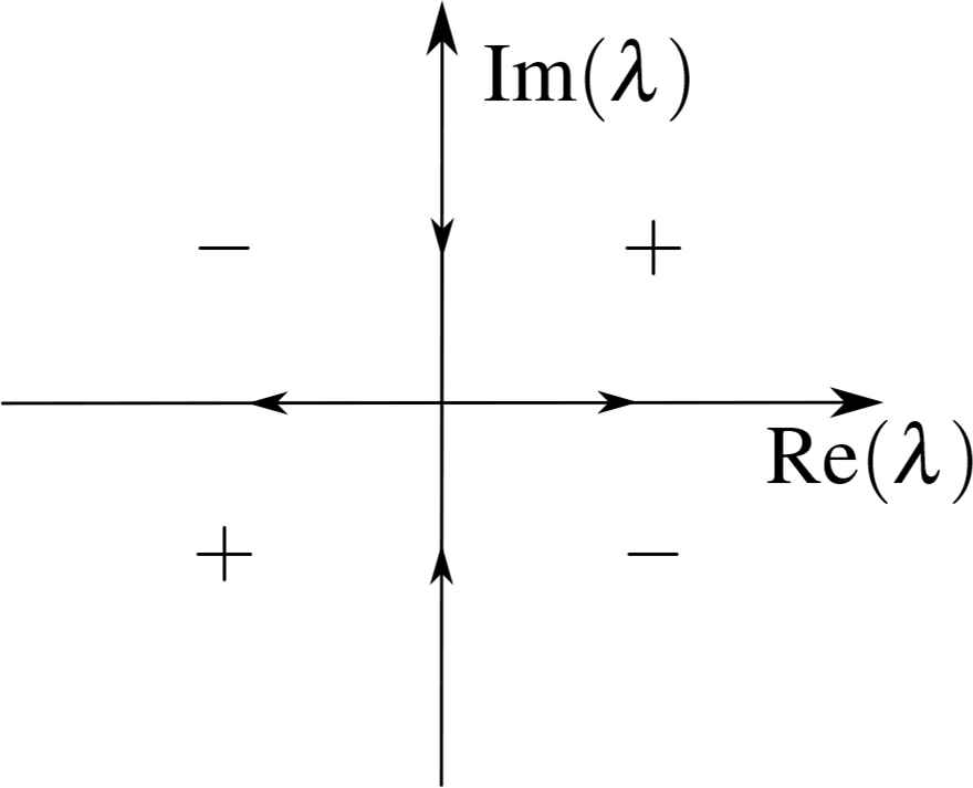
The jump contour in the complex λ-plane.
We define
From the Abel’s identity and since the trace of Q satisfies tr(Q) = 0, the determinants of J± are constants for all x. Considering the boundary conditions (2.8), we have
Thus we can derive det S(λ) = 1 according to the relation (2.9). Furthermore, from (2.9), we have
Based on the analytic property of J−, s11 is analytic extension to
In order to obtain the behavior of Jost solution P + for large λ, we use the following expansion
Substituting the expansion into the spectral problem (2.6) and compare the coefficients of λ, we have
We consider the adjoint scattering problem of (2.2)
It is easy to verify that
One can check that P− is analytic in
P− is analytic in
Summarizing the above results, we have constructed two matrix functions P + and P−, that are analytic in the complex region
We now investigate the evolutions of the scattering coefficients sij. The relation (2.9) and (2.8) leads to
Then according to the evolution property (2.3) and Q → 0 as |x| → ∞, we have
Thus the elements s11, s22 are time-independent and
3. Solutions for the Riemann-Hilbert problem
Note that the transpose and conjugate of
Here † denotes the operation of transpose and complex conjugate. From the definition of P + and P−, we have the relation
It follows from the relation (2.9) that
Furthermore, from the symmetric property σ3Q σ3 = −Q and σ3Q2 σ3 = Q2, we conclude that
Thus from the definition of P±(λ), we have the symmetry relation
Applying this reduction to (2.9), then it readily implies
Thus s11(λ) is an odd function, and each zero λk of s11 is accompanied with zero −λk. For simplicity, we assume all zeros are simple and then the kernels of
Here |vk〉 = 〈. vk|†. From the relation (3.1), we have
Differentiating both sides of the first equation of (3.3) with respect to x and t, and recalling the Lax pair (1.4)-(1.5), we have
It concludes that
Based on the above analysis, we have the following theorem for the solution to the non-regular Riemann-Hilbert problem.
Theorem 1.
The solution to a non-regular Riemann-Hilbert problem (2.15) with simple zeros under the canonical normalized condition (2.11) and (2.14) is
|wk〉 is a column vector and defined by |wk〉 = Tk−1(λk) ⋯ T1(λk)|vk〉 and |vk〉 = 〈vk|†.P±. is the unique solution to the regular Riemann-Hilbert problem
where P± are analytic in
Proof. From the symmetry relation (3.2), we can suppose that simple zeros of det P + (λ) are
From the definition of A1, we construct a meromorphic matrix function
Since ±λ1 are simple zeros of detP±(λ), the matrix P+(λ)T1−1(λ) is non-singular at λ = ±λ1, and T1(λ)P−(λ) is non-singular at λ = ±λ*. In general, near the point λk, we have det P+(λ) ∼ λ − λk and det P+(λ) ∼ λ + λk near the point − λk. Similarly,
Substituting P±(λ) into (2.15), we obtain a normalized regular Riemann-Hilbert problem (3.6).
From the above properties of Tk(λ), we could readily obtain the explicit expression for the matrix Tk(λ) (cf. Ref. [13])
4. Soliton solutions
Based on the above analysis, we are ready to construct N-soliton solutions for the higher-order CLL equation (1.3). From the asymptotic expansion of Jost solutions as λ → ∞, the potential q can be expressed as (2.12). From the expression of
Meanwhile, considering the symmetry relation Tk(−λ) = σ3Tk(λ)σ3, T(λ) and T−1(λ) have compact form
We arrive at
Solving these linear algebraic equations, we obtain
According to the Plemelj formula, the solution to the Riemann-Hilbert problem (3.6) is
From (4.1), we find T(λ) has expansion
Thus, as λ → ∞, P + (λ) = P + (λ)T(λ) has the expansion formula
In the reflection-less case, that is G = I, we obtain N-soliton solutions from (2.12). The formula for N-soliton solution is
To obtain the explicit formulae for N-soliton solutions, we take
In what follows, we shall investigate the properties of the single, two- and N-soliton solutions.
4.1. One and two-soliton solution
To obtain one-soliton solution, we set
When we take c1 = 1, one-soliton solution yields the form
Here the subscripts R and I denote the real and imaginary part of θ1, respectively. We can separate the real and imaginary parts of θ1 as
Thus the velocity for the single soliton is

(Color online) One-soliton solution for |q|.
The two-soliton solution with parameters

(Color online) Profile for interaction of two solitons.
4.2. Interactions between N -solitons
In order to analyze the N-soliton solution interactions with the variations of corresponding positions and amplitudes, we assume v1<v2<⋯<vN and keep x−vkt = constant with
Theorem 2.
Assuming
Proof. When
Thus, when t → + ∞
In the vicinity Ωk, we have
By use of the Laplace expansion and the determinant formula of Cauchy matrix, we conclude that in the vicinity Ωk, q has the asymptotic behaviour as
Similarly, when t → −∞, we can prove
Thus we have the result that on the whole plane
From the asymptotic behaviour of N-soliton solution, we know that the interaction of N solitons is elastic and only phase shifts and displacements happen.
5. Conclusion and discussion
The inverse scattering method has been applied to the higher-order CLL equation and by considering the associated Riemann-Hilbert problem, we successfully give a simple representation for the N-soliton in the determinant form. In the context we only consider the simple zeros for of the scattering matrix. The much more general case with multiple zeros would lead to more solutions. Here we only consider solutions with vanishing boundary conditions.
Because {±λj} appear simultaneously as zeros of det P +, we can assume that detP + has 2N simple zeros
In this paper, we give explicit soliton solutions to a higher-order CLL equation in the determinant form. We know that the whole NLS hierarchy could be reduced from the (extended) KP hierarchy and soliton solutions can be obtained by using the reduction method. It is deserved to compare soliton formulas obtained here with the tau function formalism.
A third problem is how to adjust the analysis and seek the Jost solutions of the spectral problem so that solutions with non-vanishing boundary conditions can be obtained. The global well-posedness, long-time behavior and asymptotic stability of solitons are left for future studies.
6. Acknowledgements
Authors appreciate the referees for their valuable suggestions. The work is supported by
References
Cite this article
TY  - JOUR
AU  - Juan Hu
AU  - Jian Xu
AU  - Guo-Fu Yu
PY  - 2021
DA  - 2021/01/06
TI  - Riemann-Hilbert approach and N-soliton formula for a higher-order Chen-Lee-Liu equation
JO  - Journal of Nonlinear Mathematical Physics
SP  - 633
EP  - 649
VL  - 25
IS  - 4
SN  - 1776-0852
UR  - https://doi.org/10.1080/14029251.2018.1503443
DO  - 10.1080/14029251.2018.1503443
ID  - Hu2021
ER  -