Journal of Nonlinear Mathematical Physics

Volume 25, Issue 1, February 2018, Pages 34 - 53

On Decomposition of the ABS Lattice Equations and Related Bäcklund Transformations

Authors
Danda Zhang, Da-jun Zhang*
Department of Mathematics, Shanghai University, Shanghai, 200444, People’s Republic of China
*Corresponding author. djzhang@staff.shu.edu.cn
Corresponding Author
Da-jun Zhang
Received 10 May 2017, Accepted 7 August 2017, Available Online 6 January 2021.
DOI
10.1080/14029251.2018.1440741How to use a DOI?
Keywords
ABS list; decomposition; Bäcklund transformation; solutions; weak Lax pair
Abstract

The Adler-Bobenko-Suris (ABS) list contains scalar quadrilateral equations which are consistent around the cube, and have D4 symmetry and tetrahedron property. Each equation in the ABS list admits a beautiful decomposition. We revisit these decomposition formulas and by means of them we construct Bäcklund transformations (BTs). BTs are used to construct lattice equations, their new solutions and weak Lax pairs.

Copyright
© 2018 The Authors. Published by Atlantis Press and Taylor & Francis
Open Access
This is an open access article distributed under the CC BY-NC 4.0 license (http://creativecommons.org/licenses/by-nc/4.0/).

1. Introduction

It is well known that discrete integrable systems play important roles in variety of areas such as statistic physics, discrete differential geometry and discrete Painlevé theory. Quadrilateral equations are partial difference equations defined on four points (see Fig. 1(a)), with a form

Q(u,u˜,u^,u˜^;p,q)=0, (1.1)
where u is a function of discrete variables n, m, constants p, q serve as spacing parameters of n-direction and m-direction, respectively. Short hand notations
u=un,m,u˜=un+1,m,u^=un,m+1,u˜^=un+1,m+1
will be used in the paper. When we speak of consistency-around-the-cube property of the quadrilateral equation (1.1), we mean that [10,21]: (i) equation (1.1) is affine linear, (ii) imposing on the six faces of the cube (see Fig. 1(b)) six equations of type (1.1),
Q(u,u˜,u^,u˜^;p,q)=0,Q(u¯,u˜¯,u^¯,u˜^¯;p,q)=0,Q(u,u˜,u¯,u˜;p,r)=0,Q(u^,u˜^,u¯^,u¯˜^;p,r)=0,Q(u,u^,u¯,u¯^;q,r)=0,Q(u˜,u^˜,u¯˜,u¯^˜;q,r)=0, (1.2)
where shift in the third direction is denoted by bar and r is spacing parameter of the third direction, one first solves the doubly shifted quantities from the left hand side of (1.2) and then the triply shifted quantity obtained from the right hand side of (1.2) are the same. In a beautiful paper [1] Adler Bobenko and Suris (ABS) classified all quadrilateral equations with the assumption of consistency-around-the-cube and additional conditions: (i) equation (1.1) having D4 symmetry; (ii) tetrahedron property, i.e. the final value of u¯˜^ only depends on u˜,u^,u¯ . ABS list includes all such consistent-around-the-cube (CAC) equations:
H1:(u-u˜^)(u˜-u^)-p+q=0, (1.3a)
H2:(u-u˜^)(u˜-u^)-(p-q)(u+u˜+u^+u˜^+p+q)=0, (1.3b)
H3(δ):p(uu˜+u^u˜^)-q(uu^+u˜u˜^)+δ(p2-q2)=0, (1.3c)
A1(δ):p(u+u^)(u˜+u˜^)-q(u+u˜)(u^+u˜^)-δ2pq(p-q)=0, (1.3d)
A2:p(1-q2)(uu˜+u^u˜^)-q(1-p2)(uu^+u˜u˜^)-(p2-q2)(1+uu˜u^u˜^)=0, (1.3e)
Q1(δ):p(u-u^)(u˜-u˜^)-q(u-u˜)(u^-u˜^)+δ2pq(p-q)=0, (1.3f)
Q2:p(u-u^)(u˜-u˜^)-q(u-u˜)(u^-u˜^)+pq(p-q)(u+u˜+u^+u˜^-p2+pq-q2)=0, (1.3g)
Q3(δ):p(1-q2)(uu^+u˜u˜^)-q(1-p2)(uu˜+u^u˜^)-(p2-q2)(u˜u^+uu˜^+δ2(1-p2)(1-q2)4pq)=0, (1.3h)
Q4:sn(p)(uu˜+u^u˜^)-sn(q)(uu^+u˜u˜^)-sn(p-q)(u˜u^+uu˜^)+sn(p)sn(q)sn(p-q)(1+k2uu˜u^u˜^)=0, (1.3i)
where δ is an arbitrary parameter, sn(p) = sn(p ; k) is the Jacobi elliptic function and Q4 in the above form was given by Hietarinta [9].

Fig. 1.

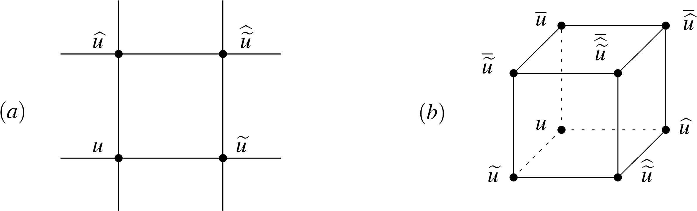
(a). An elementary quadrilateral. (b). The consistency cube.

If the top equation in the consistency cube is viewed as same as the bottom equation but with u¯ as a new solution, then the side equations as a coupled system, i.e.

Q(u,u˜,u¯,u¯˜;p,r)=0,Q(u,u^,u¯,u¯^;q,r)=0, (1.4)
automatically provides a Bäcklund transformation (BT) for the bottom equation (1.1). Its linearized form obtained by introducing u¯=g/f can act as a Lax pair of equation (1.1). The equations on the bottom and top faces have the same form at the beginning, but if one imposes different limits on the top and bottom variables then the resulting equations will be different and the two side equations will give a BT of the two resulting equations. This beautiful idea was demonstrated in [3] by Atkinson. Usually by an auto-BT we mean it connects different solutions of same equation while by a nonauto-BT we mean it connects solutions of two different equations.

BT originated from the construction of pseudo-spherical surfaces and BTs have been playing important roles in soliton theory [15,22,23]. In this paper, we will consider the ABS list and focus on those BTs that can be constructed by using decomposition property of the ABS equations. In fact, each equation Q = 0 in the ABS list admits a decomposition which is an analogue of the following,

𝒣=h12h34-h13h24=PQ,P=|QQu1Qu4Qu2Qu1u2Qu2u4Qu3Qu1u3Qu3u4|, (1.5)
where u1 = u, u2=u˜ , u3=u^ , u4=u˜^ ,
hij(ui,uj)=QukQul-QQukul, (1.6)
Quk=ukQ,Quiuk=uiukQ
, and i, j, k, l are distinct elements in {1,2,3,4}. The decomposition (1.5) played a crucial role in the classification of the ABS list and in the further discussions under the CAC property with a more general setting (allowing the faces of the consistency cube to carry a priori different quad-equations) [2,7,8]. hij are used to study singularity structures of solutions, which is considered to be related to the CAC property and boundary value structures (cf. [4,5]). The decomposition (1.5) and h polynomials can be used to construct BTs. For example, H3(δ) has the following decomposition:
𝒣=h(u,u˜,p)h(u^,u˜^,p)-h(u,u^,q)h(u˜,u˜^,q)=H3(δ)=0,
where h is defined by h(u,u˜,p)=uu˜+pδ . This implies that with unknown function U, the pair
h(u,u˜,p)=UU˜,h(u,u^,q)=UU^ (1.7)
will provide a BT to connect H3(δ) and the U -equation which comes from compatibility of the pair in terms of u. By calculation one can find the corresponding U -equation is H3(− δ). In this paper we will examine system (1.7) for some ABS equations. As a result, when h is affine linear, a completed list of BTs together with connected CAC equations are given. When h is beyond affine linear, some quadratic CAC equations are obtained. Some BTs are used to construct new solutions and weak Lax pairs.

The paper is organized as follows. In Sec. 2 we revisit decomposition of the ABS list. In Sec. 3 we discuss possible forms of h and the related quadrilateral equations of u and U, which are listed in Table 1 and 2. Sec. 4 includes some examples as applications, a new weak Lax pair of Q1(0), new polynomial solutions of Q1(δ) and rational solutions of H3*(δ) in Casoratian form are obtained. Finally, Sec. 5 is for conclusions.

No. BT(3.1) u-equation U-equation
1 1p(u-u˜)=UU˜ Q1(0, p2, q2) lpmKdV
2 u+u˜+p=UU˜ H2 H1(2p;2q)
3 1p(u+u˜)-δp=UU˜ A1(δ, p2, q2) H3(δ;2p;2q)
4 uu˜+δp=UU˜ H3(δ) H3(− δ)
5 1p(uu˜-1)=UU˜ (A.11) H3(1) with UU− 1
6 11-p2(1-puu˜)=UU˜ A2 A2(1-p2,1-q2)
Table 1.

Consistent triplets.

No. BT(3.1) u-equation U-equation
1 1n(u˜-u)2-δ2p=UU˜ Q1(δ) H3*(δ;1p,1q)
2 1p(u˜+u)2-δ2p=UU˜ A1(δ) H3*(δ;1p,1q)
3 (puu˜-1)(uu˜-p)(1-p2)uu˜=UU˜ A2 A2*(2(p2+1)1-p2,2(q2+1)1-q2)
4 (uu˜+δp)uu˜=UU˜ H3(δ) H3*(δ;4p2,4q2)
5 uu˜-ppuu˜-1=UU˜ A2 A2
6 uu˜-p(puu˜-1)uu˜=UU˜ A2 A2*(2p2-1,2q2-1)
Table 2.

BT(3.1) related to Q1(δ), A1(δ), H3(δ) and A2.

2. Decomposition (1.5) of the ABS list

2.1. Decomposition (1.5): revisited

Let us revisit the decomposition (1.5) and have a look at the relation of Q and P from a general viewpoint. Consider Q(u,u˜,u^,u˜^;p,q) to be a general quadrilateral affine linear polynomial:

Q(u,u˜,u^,u˜^;p,q)=kuu˜u^u˜^+l1uu˜u^+l2uu˜u˜^+l3uu^u˜^+l4u˜u^u˜^+p1uu˜+p2u˜u^+p3u^u˜^+p4uu˜^+p5uu^+p6u˜u˜^+q1u+q2u˜+q3u^+q4u˜^+c, (2.1)
where k, li, pi, qi, c are constants. Let 𝒫st denote a set of polynomials with s distinct variables in {u,u˜,u^,u˜^} and at most degree t for each variable. With this definition, the most general element in 𝒫41 is Q defined in (2.1) and hij belongs to 𝒫22 . For the above generic Q, the decomposition (1.5) holds and P𝒫41[2] . In fact, the discriminant of hij plays an important role in the classification of integrable quadrilateral equations. With a more general setting in the CAC condition, the classification of Q -type equations was done in [2] and a full classification was finished in [7,8].

In the following let us take a close look at the relation between Q and P in (1.5). Similar to (1.6) we define

gij(ui,uj)=PukPul-PPukul, (2.2)
where P is defined in (1.5). Then we have the following.

Proposition 2.1.

For the polynomial Q given in (2.1), P defined in (1.5) and hij in (1.6), there is a constant K such that

gij=(-1)j-iKhij,(i,j){(1,2),(1,3),(2,4),(3,4)}.

In particular when K = 0, P can be factorized as a product of distinct linear function ai ui + bi.

Proof. It has been proved that P𝒫41 [2]. Thus we can switch the roles of Q and P in (1.5). For the polynomial Q given in (2.1), P defined in (1.5) and hij in (1.6), by direct calculation we find

gij=(-1)j-iKhij,(i,j){(1,2),(1,3),(2,4),(3,4)}, (2.3)
with a same K which is an irreducible rational function of {ui}. This implies
g12g34-g13g24=K2QP.

Corresponding to the structure in (1.5), there must be

K2Q=|PPu1Pu4Pu2Pu1u2Pu2u4Pu3Pu1u3Pu3u4|𝒫41.

Since Q𝒫41 the only choice for K is a constant.

If K = 0, then we have gij = 0 in light of (2.3). Noticing that

(lnP)ukul=gijP2,
if gij = 0 we have
lnP=ψ1(u1)+ψ2(u2)+ψ3(u3)+ψ4(u4),
where ψi(ui) is a function of ui. This means P𝒫41 can be factorized as
P=φ1(u1)φ2(u2)φ3(u3)φ4(u4),
where there must be ϕi(ui) = aiui + bi because of P𝒫41

The above proposition reveals an “adjoint” relation between Q and P if Q is an affine-linear quadrilateral polynomial (2.1). For A-type and Q-type ABS equations, one can see that Q and P are almost same.

2.2. Decomposition of the ABS list

For each equation (1.1) in the ABS list it holds that [1]

𝒣=h(u,u˜,p)h(u^,u˜^,p)-h(u,u^,q)h(u˜,u˜^,q)=0, (2.4)
where function h(u,u˜,p) is h12 divided by certain factor κ(p, q). Functions, h, and connections with the ABS equations are listed below:
H1:h(u,u˜,p)=1,𝒣=0,identity, (2.5a)
H2:h(u,u˜,p)=u+u˜+p,𝒣=H2(u,u˜,u^,u˜^;p,q)=0, (2.5b)
H3:h(u,u˜,p)=uu˜+pδ,𝒣=H3(u,u˜,u^,u˜^;p,q)=0, (2.5c)
A1:h(u,u˜,p)=1p(u˜+u)2-δ2p,𝒣=A1(u,u˜,u^,u˜^;p,q)A1(u,u˜,u^,u˜^;p,-q)=0, (2.5d)
A2:h(u,u˜,p)=(puu˜-1)(uu˜-p)1-p2,𝒣=A2(u,u˜,u^,u˜^;p,q)A2(u,u˜,u^,u˜^;p,q-1)=0, (2.5e)
Q1:h(u,u˜,p)=1p(u˜-u)2-δ2p,𝒣=Q1(u,u˜,u^,u˜^;p,q)Q1(u,u˜,u^,u˜^;p,-q)=0, (2.5f)
Q2:h(u,u˜,p)=1p(u˜-u)2-2p(u+u˜)+p3,𝒣=Q2(u,u˜,u^,u˜^;p,q)Q2(u,u˜,u^,u˜^;p,-q)=0, (2.5g)
Q3:h(u,u˜,p)=p1-p2(u2+u˜2)-1+p21-p2uu˜+(1-p2)δ24p,𝒣=Q3(u,u˜,u^,u˜^;p,q)Q3(u,u˜,u^,u˜^;p,q-1)=0, (2.5h)
Q4:h(u,u˜,p)=-1sn(p)(k2sn2(p)u2u˜2+2sn(p)uu˜-u2-u˜2+sn2(p)),𝒣=Q4(u,u˜,u^,u˜^;p,q)Q4(u,u˜,u^,u˜^;p,-q)=0, (2.5i)

We note that for the ABS equations, the case K = 0 in Proposition 2.1 corresponds to H-type equations in the ABS list; for H-type equations P is a constant and for H1 even P = 0; for A-type and Q-type equations, Q and P differ only in the parameter q.

3. Bäcklund transformations

In Section 1 by H3(δ) as an example we have illustrated its decomposition can be used to construct a BT. Motivated by the decomposition (2.5) of the ABS equations, we consider the following system

h(u,u˜,p)=UU˜, (3.1a)
h(u,u^,q)=UU^, (3.1b)
where to meet the consistency w.r.t. u we request U satisfies certain quadrilateral equation
F(U,U˜,U^,U˜^;p,q)=0, (3.2)
which we call U -equation for convenience. In fact, on one hand, since u must be well defined by (3.1), the two equations in (3.1) must be compatible (i.e. u˜^=u^˜ ), which leads to the U -equation. On the other hand, for arbitrary U the function h defined by (3.1) satisfies (2.4). In a more general case, considering the following pair
h(u,u˜,U,U˜,p)=0,h(u,u^,U,U^,q)=0, (3.3)
if without knowing any information of u -equation (1.1), only by the compatibility u˜^=u^˜ we can eliminate u from (3.3) to get U -equation (3.2), and vice versa, to get u -equation (1.1), we call (3.3) and the related u -equation (1.1) and U -equation (3.2) a consistent triplet generated by (3.3) (cf. [24]). Obviously, such a consistent triplet is nothing but a special case of BTs.

As for generating solutions, we note that for H2 and H3, u solved from (3.1) with corresponding h’s will provide a solution to these two equations, while for the rest equations in the ABS list there is uncertainty. For example, for Q1, we do not know whether u solves Q1 or Q1(u,u˜,u^,u˜^;p,-q)=0 . In this section, instead of finding solutions, we are more interested in considering (3.1) as a BT to connect u-equation (2.4) and U -equation. In the following subsections Sec. 3.1, 3.2, we start from a generic affine-linear polynomial

h(u,u˜,p)=s0(p)+s1(p)u+s2(p)u˜+s3(p)uu˜, (3.4)
where si(p) are functions of p, and then examine all possibility that admits a consistent triplet in which both u-equation and U-equation are CAC. We note that h = 0 with (3.4) is a discrete Riccati equation, and the special case s1 = s2 with s3 = 0 was already considered in [3].

3.1. Consistent triplets

When h is defined as (3.4), for the relation of h and possible forms of u-equation and U -equation, we have the following.

Theorem 3.1.

When h(u, u˜ , p) in system (3.1) is defined by (3.4), then U-equation (3.2) is affine-linear if and only if either

h(u,u˜,p)=s0(p)+s1(p)u+s2(p)u˜ (3.5)
or (after a constant shift u → u − c)
h(u,u˜,p)=s0(p)+s3(p)uu˜. (3.6)

Proof. When h(u, u˜ , p) is defined by (3.4), we solve out from (3.1) that

u˜=UU˜-s0(p)-s1(p)us2(p)+s3(p)u,u^=UU^-s0(q)-s1(q)us2(q)+s3(q)u.

From the consistency u˜^=u^˜ , we have the resulting equation for U:f(U,U˜,U^,U˜^,u)=0 , which should be independent of u. Therefore the coefficient of u in f should be zero, which leads to

s2(q)s3(p)-s3(q)s1(p)=s2(p)s3(q)-s3(p)s1(q)=0. (3.7)

When s3 = 0, (3.4) turns to be (3.5). In this case, the system (3.1) is a BT for u -equation

s0(p)+s1(p)u+s2(p)u˜s0(q)+s1(q)u+s2(q)u^=s0(q)+s1(q)u˜+s2(q)u˜^s0(p)+s1(p)u^+s2(p)u˜^ (3.8)
and U -equation
U(s1(q)U˜-s1(p)U^)+U˜^(s2(q)U^-s2(p)U˜)+s0(q)(s1(p)+s2(p))-s0(p)(s1(q)+s2(q))=0. (3.9)

Here we note that equation (3.8), (3.9) and the BT (3.1) compose a consistent triplet (cf.[24]), i.e. viewing the BT(3.1) as a two-component system, then the compatibility of each component yields a lattice equation of the other component which is in the triplet.

When function s3 ≠ 0, we have

c=s2(q)s3(q)=s1(p)s3(p)=s1(q)s3(q)=s2(p)s3(p),
where c is a constant independent of p and q. It then follows that s2 = s1 = c s3. Thus (3.4) yields
h(u,u˜,p)=s0(p)-c2s3(p)+s3(p)(u+c)(u˜+c),
which then reduces to (3.6) by redefine s0(p) → s0(p) + c2 s3(p) and uuc. Consequently the u-equation reads
(s0(p)+s3(p)uu˜)(s0(p)+s3(p)u˜u˜^)=(s0(q)+s3(q)uu^)(s0(q)+s3(q)u˜u˜^) (3.10)
and U -equation reads
(s32(p)-s32(q))UU˜U^U˜^+U(s0(p)s32(q)U˜-s0(q)s32(p)U^)+U˜^(s0(p)s32(q)U^-s0(q)s32(p)U˜)=s02(p)s32(q)-s02(q)s32(p). (3.11)

Note that replacing s0 with -s0s3 and s3 with 1s3 , equation (3.10) becomes (3.11). Eqs. (3.10), (3.11) and (3.1) compose a consistent triplet as well.

Now we have obtained four quadrilateral equations, (3.8), (3.9), (3.10) and (3.11), all of which are derived as a compatibility of (3.1). Among them, equation (3.8) with s0 = 1, s1(p) = pa, s2(p) = p + a can be considered as the Nijhoff-Quispel-Capel (NQC) equation with b = a(cf. [19] and eq. (9.49) in [10]).

3.2. CAC property with h given in (3.5) and (3.6)

Although (3.8), (3.9), (3.10) and (3.11) are derived as a compatibility of (3.1), it is not true that they are CAC for arbitrary si. After a case-by-case investigation of the CAC property of the four equations, we reach a full list that includes all CAC equations when h are given in (3.5) and (3.6) which is presented in the following theorem:

Theorem 3.2.

For the system (3.1) where h is affine-linear as given in (3.5) and (3.6), if it generates a consistent triplet and acts as a BT between quadrilateral equations which are CAC, the exhausted results are

Proof of the theorem is given in Appendix A.

Here we have two remarks. First, most of the BTs in Table 1 can be found from known literatures. For example, transformation 1 was already known in [16,18,20] as a BT connecting the lattice Schwarzian KdV (Q1(0)) equation and lpmKdV equation, transformation 2 and 3 were given in [3], transformation 6 can be found from eq. (57) of [6] by first taking (A, B, C) = (1,0,0), then (0,0,1) and next eliminating s, t from the obtained equations, transformation 4 can be found from eq. (58) of [6] by first taking (A, B, C) = (0,1,0), then (0,0,1) and next eliminating s, t from the obtained equations. The second remark is although transformation 1 is a special case of 3 by taking δ = 0 and imposing a point transformation, we would like to keep it in the table because it does not only connect the lattice Schwarzian KdV equation and lpmKdV equation but also plays a practical role in deriving lattice equations in Cauchy matrix approach [17] as well as in generating rational solutions [24].

3.3. Other cases: Q1(δ), A1(δ) and A2

For equations Q1(δ), A1(δ) and A2, their h polynomials are not affine linear. We discuss them one by one.

First, for Q1(δ), the corresponding system (3.1) is

(u˜-u)2-δ2p2=pUU˜,(u^-u)2-δ2q2=qUU^, (3.12)
which is quadratic w.r.t. u. We find if u satisfies Q1(δ), then U satisfies
[p(UU˜-U^U˜^)-q(UU^-U˜U˜^)]2+4pq(U˜-U^)[δ2(p-q)(U-U˜^)-UU˜^(U˜-U^)]=0, (3.13)
and vice versa. The above equation can be transformed to H3*(δ) equation
(p-q)[p(UU^-U˜U˜^)2-q(UU˜-U^U˜^)2](U-U˜^)(U˜-U^)[(U-U˜^)(U˜-U^)pq-4δ2(p-q)]=0, (3.14)
by transformation p → 1 / p, q → 1 / q. Here we note that H3*(δ) is one of integrable quad equations that are multi-quadratic counterparts of the ABS equations. These multi-quadratic equations are consistent in multi-dimensions as well and were systematically found in a beautiful work [6]. System (3.12) provides a BT between Q1(δ) and H3*(δ) (3.13).

Similarly, for A1, we find

(u˜+u)2-δ2p2=pUU˜,(u^+u)2-δ2q2=qUU^, (3.15)
provides a BT between A1 and H3*(δ) (3.13).

For A2, in the system (3.1) there is

h(u,u˜,p)=(puu˜-1)(uu˜-p)1-p2. (3.16)

It is hard to write out a U -equation in a neat form. However, by observing that U is arbitrary in (3.1), we can replace U with U / f(u) where f(u) is a suitable function of u so that the deformed BT

h(u,u˜,p)f(u)f(u˜)=UU˜,h(u,u^,q)f(u)f(u^)=UU^ (3.17)
generates a U -equation with an explicit and neat form. Taking f(u) = 1 / u, (3.1) with (3.16) becomes
(puu˜-1)(uu˜-p)(1-p2)uu˜=UU˜,(quu^-1)(uu^-q)(1-q2)uu^=UU˜, (3.18)
which connects the solutions between A2(u) and A2*(U) equation [6]
(p-q)[p(UU^-U˜U˜^)2-q(UU˜-U^U˜^)2]+(U-U˜^)(U˜-U^)[(U-U˜^)(U˜-U^)(pq-1)+2(p-q)(1+UU˜U^U˜^)]=0, (3.19)
with p → 2(p2 + 1) /(1−p2), q → 2(q2 + 1) /(1 − q2). One more example of utilizing f(u) is H3(δ). For the transformation 4 in Table 1, taking f(u) = u we have
(uu˜+δp)uu˜=UU˜,(uu^+δq)uu^=UU^, (3.20)
which connects the solutions between H3(δ)(u) and H3 *(δ)(U) equation with parameters p → 4 / p2, q → 4 / q2. BTs (3.18) and (3.20) have been listed in [6]. Let us look at a third example. It can be verified that
uu˜-ppuu˜-1=UU˜,uu˜-qquu˜-1=UU^ (3.21)
is an auto-BT of A2. Taking f(u) = 1 / u the new BT provides a transformation between A2(u) and A2*(U) with parameters p → 2 p2−1, q → 2 q2−1.

We collect the BTs obtained in this subsection in Table 2.

In this section we have given an exhausted examination for the case where h is the affine-linear polynomial (3.4). For Q1(δ), A1(δ) and A2, their h polynomials are not affine linear and their corresponding U -equations are usually multi-quadratic counterparts of the ABS equations, (see Table 2). For Q2, Q3 and Q4, their h polynomials are so complicated that from system (3.1) we can not derive explicit U -equations.

We also note that there are many systematical works to consider constructions of BTs for quadrilateral equations [3,6,13,14]. In [6] many BTs are constructed by considering compatibility of (3.3) which are Riccati equations in terms of U but allowing more freedom for u. Besides, [6] presents variety of BTs with free parameters (A, B, C) that are derived by using Yang-Baxter maps. BTs in Table 2 are included in the results of [6].

4. Applications

BTs have been used as a main tool to find rational solutions for quadrilateral equations (see [24]). In this section we would like to introduce more applications, including a BT and weak Lax pair of Q1(0), polynomial solutions of Q1(δ) and rational solutions of H3*(δ).

4.1. BT and weak Lax pair of Q1(0)

From the previous discussion, we know that Q1(0),

p2(u-u^)(u˜-u˜^)-q2(u-u˜)(u^-u˜^)=0, (4.1)
has a BT
u˜-u=pUU˜,u^-u=qUU^, (4.2)
where U satisfies the lpmKdV equation. If U solves the lpmKdV equation, so does 1 / U. Employing this symmetry we introduce
u¯˜-u¯=pU-1U˜-1,u¯^-u¯=qU-1U^-1 (4.3)
as an adjoint system of (4.2), which is also a BT between Q1(0) and lpmKdV. Eliminating U from (4.2) and (4.3) we reach
(u¯˜-u¯)(u˜-u)=p2,(u¯^-u¯)(u^-u)=q2,
which gives an auto-BT of Q1(0). Noticing the symmetry that u and 1 / u can solve Q1(0) simultaneously, we replace u¯ with 1/u¯ and reach
(u¯˜-u¯)(u˜-u)+p2u¯u¯˜=0,(u¯^-u¯)(u^-u)+q2u¯u¯^=0, (4.4)
which gives another auto-BT of Q1(0). One can check that the following 6 equations
p2(u-u^)(u˜-u˜^)-q2(u-u˜)(u^-u˜^)=0, (4.5a)
(u¯˜-u¯)(u˜-u)+p2u¯u¯˜=0, (4.5b)
(u¯^-u¯)(u^-u)+q2u¯u¯^=0, (4.5c)
(u¯˜^-u¯^)(u˜^-u^)+p2u¯^u¯˜^=0, (4.5d)
(u¯˜^-u¯˜)(u˜^-u˜)+q2u¯˜u¯˜^=0, (4.5e)
p2(u¯-u¯^)(u¯˜-u¯˜^)-q2(u¯-u¯˜)(u¯^-u¯˜^)=0 (4.5f)
can be consistently embedded on 6 faces of a cube.

The BT (4.3) yields a pair of linear problems (Lax pair):

Φ˜=(10p2u˜-u1)Φ,Φ^=(10q2u^-u1)Φ, (4.6)
where Φ = (g, f)T. The consistency of (4.6) leads to an equation
(u-u˜-u^+u˜^)[p2(u-u^)(u˜-u˜^)-q2(u-u˜)(u^-u˜^)]=0, (4.7)
which is Q1(0) multiplied by a factor (u-u˜-u^+u˜^) . This means Q1(0) can not be fully determined by (4.6). Such an Lax pair is called a weak Lax pair and was first systematically studied in [11]. (4.6) is a new weak Lax pair of Q1(0). As a result, replacing (4.5a) and (4.5f) by
u-u˜-u^+u˜^=0,u¯u¯˜u¯^u¯˜^(1/u¯-1/u¯˜-1/u¯^+1/u¯˜^)=0,
respectively, (4.5) is also consistent around the cube as a system.

In addition to the weak Lax pair of Q1(0), we have shown an approach to construct auto-BT for u -equation from (3.1) if U -equation admits a symmetry U → 1 / U. For A2 and related BT (3.21), employing the same technique, we have relations

(uu˜-p)(u¯u¯˜-p)=(puu˜-1)(pu¯u¯˜-1),(uu^-q)(u¯u¯^-q)=(quu^-1)(qu¯u¯^-1),
and
(uu˜-p)(1-pu¯u¯˜)=(puu˜-1)(p-u¯u¯˜),(uu^-q)(1-qu¯u¯^)=(quu^-1)(q-u¯u¯^).

Both of them are auto BTs of A2.

4.2. Polynomial solutions of Q1(δ)

Consider (3.12), i.e.

(u˜-u)2-δ2p2=pUU˜,(u^-u)2-δ2q2=qUU^, (4.8)
which is a BT between Q1(δ) and H3*(δ). However, if we do not care about what U -equation is, then from decomposition (2.5f) any u defined by (4.8) will be a solution of
𝒣=Q1(u,u˜,u^,u˜^;p,q)Q1(u,u˜,u^,u˜^;p,-q)=0. (4.9)

In other words, (4.8) may also be a BT between Q1(u,u˜,u^,u˜^;p,-q)=0 . and some U -equation other than H3(δ). This means, if we just solve (4.8) and obtain u, we should verify whether u satisfies Q1(δ) (1.3f) or Q1(u,u˜,u^,u˜^;p,-q)=0 .

To solve (4.8) which is a quadratic system, we suppose that U is a polynomial of

x=an+bm+γ, (4.10)
say,
U=i=0NcN-ixi (4.11)
with constants a, b, γ, ci and c0 ≠ 0, N ≥ 0. Introduce
v1=u˜-u,v2=u^-u, (4.12)
where v1 and v2 should satisfy
v^1-v1=v˜2-v2 (4.13)
due to consistency of (4.12). For the case that both v1 and v2 are also polynomials of x, we have the following result:

Theorem 4.1.

When U is given in (4.11), we can convert the system (4.8) to

v12-δ2p2=pUU˜,v22-δ2q2=qUU^. (4.14)

When N ≥ 1 and we require that vi have the following form,

v1=i=0NfN-ixi,v2=i=0NgN-ixi (4.15)
with constants fi, gi to be determined, the only allowed values for N are 1 and 2. u is recovered through (4.12).

The proof for this theorem is given in Appendix B.

Let us turn to find polynimial solutions. When N = 0, we have U = c0 and

(u˜-u)2=p(δ2p+c02),(u^-u)2=q(δ2q+c02).

Suppose

p=c02a2-δ2,q=c02b2-δ2,α=pa,β=qb. (4.16)

It turns out that four possibilities for u are

αn+βm+γ,(-1)n+12α+βm+γ,αn+(-1)m+12β+γ,(-1)n+12α+(-1)m+12β+γ,
which coincide with the result in [12].

When N = 1,2, with p, q parameterized as

p=a2,q=b2, (4.17)
following Theorem 4.1, after some calculation and scaling, we find solutions to (4.8):
u=±δx2+γ0,U=±2δx, (4.18a)
u=c03x3-δ2c0x-c03(a3n+b3m)+γ0,U=c0x2-δ2c0. (4.18b)

We can check that u and U respectively satisfy Q1(δ) and H3*(δ) equation (3.13). These are polynomial solutions.

4.3. Rational solutions of H3*(δ)

One can derive rational solutions for H3*(δ) from those of Q1(δ) and BT (3.12).

It has been proved that Q1(δ) with p, q parameterized as in (4.17) has the following rational solutions [24]:

uN+2=f¯¯+δ2f__f, (4.19)
where N -th order Casoratian f is given by
ffN=|N-1^|=|α(n,m,0),α(n,m,1),,α(n,m,N-1)|,
for N ≥ 1 and extended to negative direction by
f-N=(-1)[N2]fN-1,f0=1, (4.20)
[⋅] denotes the greatest integer function, f_=fN-1=|N-2^|,f¯=fN+1=|N^| , etc; the Casoratian vector α is
α(n,m,l)=(α0,α1,,αM-1)T,αj=1(2j+1)!si2j+1ψi|si=0,M=1,2,
with function ψi
ψi(n,m,l)=ψi+(n,m,l)+ψi-(n,m,l),ψi±(n,m,l)=ρi±(1±si)l(1±asi)n(1±bsi)m,
where
ρi±=±12exp[-j=1(si)jjγj],γj𝔺.

The Casoratian f defined above satisfies a superposition relation [24]

f¯¯˜f-f¯¯f˜=af¯˜f¯, (4.21a)
f¯¯^f-f¯¯f^=bf¯^f¯. (4.21b)

Making use of (3.12), (4.19), (4.20) and (4.21), by a direct calculation we find rational solutions of H3*(δ) (3.13) can be written as

UN+2=f¯2-δ2f_2f2,N𝕑. (4.22)

The first three solutions are

U1=1-x12δ2,U2=x12-δ2,U3=(x13-x3)2-9δ29x12,
where
xi=ain+bim+γi.

Here U2 is (4.18b) with c0 = 1

Finally, we note that, compared with the solution of H3(δ) given by [24], which is

uN+2=(-1)n+m2+14f¯+(-1)n+mδf_f,
when δ=i=-1 it is interesting to find the relation UN = |uN|2.

5. Conclusions

BTs contain compatibility and are closely related to integrability of the equations that they connect. In this paper we have investigated system (3.1) as a BT. When h is affine linear with a generic form (3.4), we made a complete examination and all consistent triplets are listed in Table 1. As applications, apart from constructing solutions (cf. [24]), these BTs in the triplets can be viewed as Lax pairs of u -equations, where wave function Φ = (g, f)T can be introduced by taking U = g / f but usually it is hard to introduce an significant spectral parameter. When h is beyond affine linear, system (3.1) as a BT and the connecting quadrilateral equations (including multi-quadratic ones) are listed in Table 2. Further applications of the obtained BTs, such as constructing weak Lax pair and rational solutions for multi-quadratic lattice equations, were also shown in the paper.

Acknowledgments

We are grateful to the referees and editor for their invaluable comments. This project is supported by the NSF of China (Nos. 11371241,11631007 and 11601312).

Appendix A. Proof of Theorem 3.2

A.1. Multidimensional consistency: h given in (3.5)

The following discussion is on the basis of the CAC condition u˜^¯=u¯˜^=u¯^˜ for system (1.2). First we investigate the case of (3.8) and (3.9) with h(u,u˜,p) given in (3.5) where we assume s1(p) s2(p) ≠ 0 otherwise (3.8) is not a quadrilateral equation.

A.1.1. s0 = 0

In this case, it can be verified that (3.8) always satisfies the CAC condition u˜^¯=u¯˜^=u¯^˜ . Canonically, we make a transformation u(-s1(p)s2(p))n(-s1(q)s2(q))mu so that equation (3.8) is in a neat form

s1(p)s2(p)(u-u˜)(u^-u˜^)=s1(q)s2(q)(u-u^)(u˜-u˜^).

Without any loss of generality, by assumption of s1(p)=-s2(p)=1p , equation (3.8) turns out to be the equation Q1(0; p2, q2)a, while the corresponding equation (3.9) becomes the lpmKdV equation,

p(UU˜-U^U˜^)-q(UU^-U˜U˜^)=0. (A.1)

A.1.2. s0 ≠ 0

A. s1(p) + s2(p) = ks0(p) with constant k

This goes to the case of s0 = 0 by taking uuk− 1 when k ≠ 0 and uus0(p)ns0(q)m when k = 0.

B. s1(p) + s2(p) = ks0(p) with nonconstant k

Check all terms in u˜^¯=u¯^˜ where the coefficient of uu¯3 reads

s1(p)s24(r)A(B+C), (A.2)
with
A=s2(p)s1(p)-s2(q)s1(q),B=(-s0(p)s1(p)+s0(q)s1(q))(s2(r)+s1(r)),C=(s12(p)+s2(p)s1(p)-s12(q)-s2(q)s1(q))s0(r)+[s0(p)s2(q)+s1(q)s0(p)-s1(p)s0(q)-s0(q)s2(p)]s1(p)s1(q)s2-1(r).

Letting (A.2) vanish leads to only three subcases.

Case B.1. A = 0

It directly results in

s2(p)s1(p)=c0,withconstantc0. (A.3)

Then from the coefficient of u¯3 we have

s14(p)s12(q)EF=0, (A.4)
where
E=s0(p)s1(p)(s12(q)+c0)-s0(q)s1(q)(s12(p)+c0),F=c02s1(p)s0(p)-c02s0(q)s1(q)-c0(s12(p)-s12(q))s0(r)s1(r)+(s0(q)s1(p)-s0(p)s1(q))s1(p)s1(q)s12(r).

If E = 0, it returns to the Case A. In fact, when E = 0, under (A.3) we have

s12(p)+c0s1(p)s0(p)=s12(q)+c0s1(q)s0(q)=c1=s1(p)+s2(p)s0(p),
with constant c1.

In the case that F = 0 and s1(p) is not a constant, it again returns to Case A. In fact, in this case from F = 0 we can take s0 to be the form

s0(t)=c1s1(t)+c2s1-1(t),
where c1 and c2 are constants. Substituting the above with t = p, q, r into F = 0 it turns out that c2 = c1c0, from which and (A.3) we find s1(p) + s2(p) = s0(p) / c1, which brings the case to Case A. Thus the only choice is s1(p) being a constant. Without loss of generality we suppose s1(p) = 1 and as a consequence of (A.3) we also have s2(p) = c0. Then, after checking the remaining terms in u˜^¯=u¯˜^=u¯^˜ we find c0 = 1. Therefore in this case we have h(u,u˜,p)=u+u˜+p , and (3.8) and (3.9) are nothing but H2 and H1(2p, 2q).

Case B.2. A ≠ 0, B = C = 0

B = 0 yields either s2(r) + s1(r) = 0 or s0(p)s1(p) = c0 with constant c0. The former belongs to Case A and then we consider the later, i.e.

s0(p)s1(p)=c0. (A.5)

Note that if the term s12(p)+s2(p)s1(p)-s12(q)-s2(q)s1(q) in C vanishes we will find (s1(p) + s2(p))s1(p) to be a constant, which, together with (A.5), again leads to Case A. If the term does not vanish, from C = 0 we can assume there are constants c2 and c3 such that c2s0(r)+c3s2-1(r)=0 , i.e.

s0(r)s2(r)=c1=-c3/c2. (A.6)

Making use of (A.5) and (A.6) we reach

c0(c12-c02)c1(1s02(p)-1s02(q))=0.

We ignore solution s0 = c because this leads to s1 and s2 to be constants and then brings the case to Case A. Therefore we have c1 = ±c0. Since c1 = −c0 results in k = 0 which is Case A, the only choice is c1 = c0 and in this case the canonical form for h can be

h(u,u˜,p)=1p(u˜+u)-δp.

Then it follows that (3.8) is A1(δ; p2, q2), and the corresponding (3.9) is H3(δ; 2p, 2q).

Case B.3. A B ≠ 0, B + C = 0

Since B ≠ 0, from B + C = 0 we can assume

s1(r)+s2(r)=c1s0(r)+c2s2-1(r), (A.7)
with constant c1 and nonzero constant c2(if c2 = 0 we back to Case A), in which
c1=s1(p)(s2(p)+s1(p))-s1(q)(s2(q)+s1(q))s0(p)s1(p)-s0(q)s1(q), (A.8a)
c2=[s0(p)(s2(q)+s1(q))-s0(q)(s1(p)+s2(p))]s1(p)s1(q)s0(p)s1(p)-s0(q)s1(q). (A.8b)

Note that in Case B s0(r) and s2-1(r) must be linearly independent. Separate p and q in (A.8a) we find s1(p)(s2(p) + s1(p)) − c1 s0(p)s1(p) = c0 with nonzero constant c0, which, together with relation (A.7), yields s2(p)=c2c0-1s1(p) . Now, substituting this relation and (A.7) into (A.8b) we find c2 = c0, and consequently, s1(p) = s2(p). Thus, (3.5) of this case reads

h(u,u˜,p)=s0(p)+s1(p)u+s1(p)u˜, (A.9)
and (A.7) reads
2s1(r)=c1s0(r)+c0s1-1(r).

We note that (A.9) is already discussed in [3]. After making uu−1 / c1 in (A.9) we can consider

h(u,u˜,p)=-c0c1s1(p)+s1(p)u+s1(p)u˜,
which, however, leads to Case B.2. So, nothing new is obtained in this case.

A.2. CAC property: h given in (3.6)

For h(u,u˜,p) given in (3.6), we suppose s0(p), s3(p) ≠ 0 and they are not constants simultaneously, so that we can keep the freedom of p, q. By the same manner, from the coefficient of u˜u^3 in u˜^¯=u¯^˜ , we find

s32(p)s02(r)-s32(r)s02(p)+s32(r)s02(q)-s32(q)s02(r)+s32(q)s02(p)-s32(p)s02(q)=0. (A.10)

If s3(p) is a constant, setting s3(p) = 1, s0(p) = , we have h(u,u˜,p)=uu˜+pδ , (3.10) is H3(δ) and (3.11) is H3(− δ).

If s0(p) is a constant, by setting s0(p) = 1, s3(p) = , it comes out that h(u,u˜,p)=δpuu˜+1 . By transformation uu− 1, (3.10) also reaches H3(δ).

If neither s0(p) or s3(p) is a constant, ∂pq(A.10) yields

(s02(p))(s32(p))=(s02(q))(s32(q))=c1,
which leads to s02(p)=c1s32(p)+c2 with nonzero constant c1. When c2 = 0, it yields s0(p) = δs3(p). Replacing u →(−δ)1 / 2 u and taking s3(p) = 1 / p, we can write equation (3.10) as
q2(uu˜-1)(u^u˜^-1)=p2(uu^-1)(u˜u˜^-1), (A.11)
and the corresponding (3.11) is H3(1) after transformation UU− 1. When c2 ≠ 0, we can scale c1 to be 1 by replacing u →(c1)1 / 4 u. Then, setting c2=1,s3(p)=-p1-p2,s0(p)=11-p2 , equation (3.10) reduces to A2 and (3.11) reduces to A2(1-p2,1-q2) .

We note that (A.11) is not a new equation. It is related to Q1(0; p2, q2) by uu(-1)n+m .

As a conclusion we have proved Theorem 3.2.

Appendix B. Proof of Theorem 4.1

According to the BT (4.8) and assumption (4.11) and (4.12), we can assume that vi have the following special form

v1=(-1)θ1i=0NfN-ixi,v2=(-1)θ2i=0NgN-ixi (B.1)
with constants fi, gi to be determined, where θi can be arbitrary functions of n, m. First we have the following.

Lemma B.1.

With U defined in (4.11) and v1, v2 defined above, when N ≥ 1, we have

v1=i=0NfN-ixi,v2=i=0NgN-ixi. (B.2)

Proof. Substituting (4.11) and (B.1) into system (4.8) and (4.13), from the coefficient of the leading term x2N (if N ≥ 1) in (4.8) we find

f02=c02p,g02=c02q, (B.3)
which means f02g02=pq , and from the coefficient of xN in (4.13) we find
f0((-1)θ^1-(-1)θ1)=g0((-1)θ˜2-(-1)θ2).

Consequently we have

((-1)θ^1-(-1)θ1)2p=((-1)θ˜2-(-1)θ2)2q.

Since p, q are independent constants, it follows that θ1 = θ1(n), θ2 = θ2(m). Consequently, from the coefficient of xN−1(N ≥ 1) in (4.13) we have (-1)θ1f0b=(-1)θ2g0a which leads to the fact that θ1 and θ2 are constants. Noticing that θ1 and θ2 can be absorbed into fi, gi, we can assume θ1 = θ2 = 0 without loss of generality. Thus (B.1) becomes (B.2).

Lemma B.2.

With U defined in (4.11) and v1, v2 defined in (B.2), when N ≥ 1, the allowed values of N are only 1,2.

Proof. Analyzing the coefficient of xN − 1(N ≥ 1) in (4.13), we obtain f0b = g0a, which leads to a2b2=pq in light of (B.3). So we have p = θa2, q = θb2 with constant θ. θ can be scaled to be 1 using δ, therefore we set p = a2, q = b2 (i.e (4.17)) and f0 = tc0a, g0 = tc0b, t2 = 1 from (B.3). One can always take t to be 1 as system (4.8) remains invariant under U → − U. Consequently we have

f0=c0a,g0=c0b. (B.4)

Substituting (B.2), (4.17) and (B.4) into the coefficient of x2N − 1(N ≥ 1) in (4.8), we can work out

f1=2c1+c0aN2a,g1=2c1+c0bN2b. (B.5)

Then substituting (4.17)(B.5) into the coefficient of xN − 2(N ≥ 2) in (4.13), we find it varnishes. Next, analyzing the coefficient of x2N − 2(N ≥ 2) in (4.8), we have

f2=a8(8c2+4ac1(N-1)+a2c0(N2-2N)),g2=b8(8c2+4bc1(N-1)+b2c0(N2-2N)). (B.6)

Substituting (4.17)(B.6) into the coefficient of xN − 3(N ≥ 3) in (4.13), we obtain

abc0(a2-b2)(N2+2N)=0
which admits zero option if N ≥ 3. Therefore all possible choices of N can only be 1,2.

Footnotes

a

By this we denote Q1(0) in which replacing p and q by p2 and q2

References

[4]J Atkinson, Singularities of type-Q ABS equations, SIGMA, Vol. 7, 2011, pp. 14. No.073
[8]R Boll, Classification and Lagrangian structure of 3D consistent quad-equations, Technischen Universität Berlin, Berlin, 2012. Doctoral Thesis
[10]J Hietarinta, N Joshi, and FW Nijhoff, Discrete Systems and Integrablity, Camb. Univ. Press, Cambridge, 2016.
[13]P Kassotakis and M Nieszporski, Families of integrable equations, SIGMA, Vol. 7, 2011, pp. 14. No.100
[22]R Prus and A Sym, Rectilinear congruences and Bäcklund transformations: roots of the soliton theory, D Wöjcik and J Cieśliński (editors), Nonlinearity & Geometry, Polish Scientific, Warsaw, 1998, pp. 25-36. Luigi Bianchi Days Proc. 1st Non-Orthodox School (Warsaw, 21-28 Sep. 1995)
[23]C Rogers and WK Schief, Bäcklund and Darboux Transformations, Camb. Univ. Press, Cambridge, 2002.
[24]DD Zhang and DJ Zhang, Rational solutions to the ABS list: Transformation approach, Symm. Integr. Geom.: Meth. Appl., Vol. 13, 2017, pp. 24. No.078
Journal
Journal of Nonlinear Mathematical Physics
Volume-Issue
25 - 1
Pages
34 - 53
Publication Date
2021/01/06
ISSN (Online)
1776-0852
ISSN (Print)
1402-9251
DOI
10.1080/14029251.2018.1440741How to use a DOI?
Copyright
© 2018 The Authors. Published by Atlantis Press and Taylor & Francis
Open Access
This is an open access article distributed under the CC BY-NC 4.0 license (http://creativecommons.org/licenses/by-nc/4.0/).

Cite this article

TY  - JOUR
AU  - Danda Zhang
AU  - Da-jun Zhang
PY  - 2021
DA  - 2021/01/06
TI  - On Decomposition of the ABS Lattice Equations and Related Bäcklund Transformations
JO  - Journal of Nonlinear Mathematical Physics
SP  - 34
EP  - 53
VL  - 25
IS  - 1
SN  - 1776-0852
UR  - https://doi.org/10.1080/14029251.2018.1440741
DO  - 10.1080/14029251.2018.1440741
ID  - Zhang2021
ER  -