
Sticking Fault Detecting Method for CARIMA Model
- DOI
- 10.2991/jrnal.2018.5.3.1How to use a DOI?
- Keywords
- Fault detection; sticking fault; CARIMA model
- Abstract
This paper proposes a sticking fault detecting method for controlled auto-regressive integrated moving average model (CARIMA) which detect the sticking fault of control input and feedback signal. It consists of model estimation using recursive least square method with the forgetting factor and fault detection. In the fault detection, an evaluation function is introduced, and it generates a fault signal from the input and output data. Numerical simulations are performed, and it is shown that this method can detect the sticking fault.
- Copyright
- © 2018 The Authors. Published by Atlantis Press SARL.
- Open Access
- This is an open access article under the CC BY-NC license (http://creativecommons.org/licences/by-nc/4.0/).
1. INTRODUCTION
If a system with a fault continues to be operated, it can cause a serious accident or a considerable damage. Thus, it is important to detect faults and compensate them, and many fault detection methods have been proposed [1,2]. The advantage of fault detection is that the safety is improved, you can cope with the fault more promptly, and sometimes the system can be controlled compensating the fault. There are two kinds in fault detection, signal-based detection and model-based one. The signal-based detection is for example a method using spectral analysis, statistical signal analysis or pattern recognition, while the model-based detection uses an observer or a parameter estimation [3]. In model-based detection, a general method detecting additive faults is proposed by Isermann [4].
In detecting a fault where control input or feedback signal is fixed, a general detection method is not established. In this paper, we propose a model-based detection method for the sticking fault of control input and feedback signal on a system expressed as a controlled auto-regressive integrated moving average (CARIMA) model. Then, we discuss its effectiveness performing a numerical simulation.
2. STICKING FAULT DETECTING METHOD
In this section, we discuss how to detect sticking fault of control input and feedback signal on the general linear systems.
2.1. Problem Statement
First, we assume the control object is single input and single output system and expressed in Eq. (1) as following CARIMA model:
Let us define the sticking fault. When the sticking fault of control input occurs, the input to the system um(k) becomes a white noise and expressed in Eq. (2):
Figure 1 shows a block diagram of the fault detection for the above-mentioned faults. This method consists of two parts, model estimation and fault analysis.
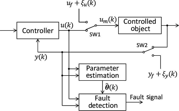
Block diagram of sticking fault detection
2.2. Model Estimation
Least square method with the forgetting factor [5] is used for the model estimation. In this method, the cost function is given in Eq. (4):
The weight of a past input–output data in cost function IN(θ) becomes smaller as the time goes by due to the forgetting factor. Thus, the estimated parameter
2.3. Fault Detection
Figure 2 shows the outline of the fault detection. To detect sticking fault, it uses the estimated system parameters and the input–output data of past nd steps called detecting period. The fault state is evaluated by the following Eq. (8):
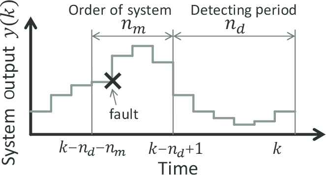
Outline of fault detection
We assume a situation that a fault has occurred. The estimated parameters become useless values after the fault. However, at a moment like Figure 2, estimated parameter
3. STICKING FAULT EVALUATION VALUE
We discuss the size of the evaluation value V(k) on the normal state and the fault one. First, let us define the error polynomials of the system parameters, EA[z−1] and EB[z−1] as Eq. (10):
On the other hand, after the sticking fault of the input has occurred, the evaluation value at a moment described in Figure 2 is deformed using Eq. (2) of the fault state and Eqs. (1), (3) and (10), and expressed as Eq. (12):
Systems usually have limitations of the control input. When designing a controller considering the limitation, higher and lower constant limits are generally used. However, Eqs. (11–13) state that Δu(i) has to have a value, and Δu(i) can be 0 when the input is limited by the constant value. Thus, the limitation has to be dependent on time, and is given by Eq. (14):
4. SIMULATION EXAMPLE
To verify the effectiveness of this fault detecting method, we apply it to a system expressed as Eq. (15):
In the model estimation, we assume that the order of the system parameter polynomials l, m and n and the time delay km are known. Then, the estimated parameter vector
Generalized predictive control [6] which uses CARIMA model to predict the output is used as a controller. When designing it, Eq. (14) is used for the internal model, and N1 = 1, N2 = 5, NU = 5, λ(j) = 0.01, and time constant of the reference trajectory τ = 0.3 s are taken. For the input limitation, A = 1, ω = 0.1π, uh = 4 and ul = −4 are used.
Figure 3 shows a simulation result where the sticking fault of control input occurs at a step 400. r(k) represents reference value and the dashed line on the graph V(k) is the threshold value Vth. The evaluate value V(k) is normally smaller than 1, and it becomes greater after the fault occurs. It surpasses Vth at a step 406, and then the fault signal is generated. V(k) takes relatively great value on the beginning due to the error of the parameter estimation.
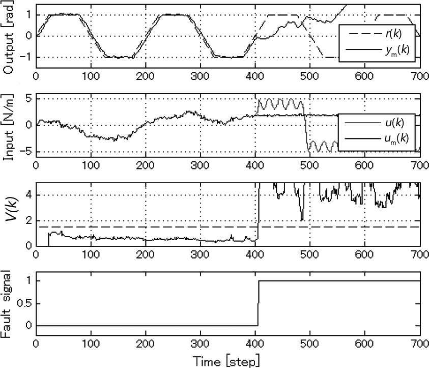
Detection result on control input sticking fault
Figure 4 shows a result of the sticking fault of feedback signal. Like Figure 3, V(k) becomes greater after the fault, and the fault signal is generated at a step 404.
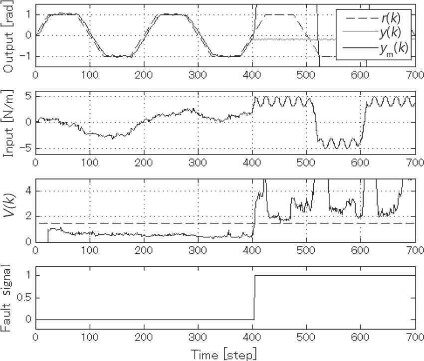
Detection result on feedback sticking fault
5. CONCLUSION
We proposed the sticking fault detecting method in which the evaluation function is introduced. It evaluates the input–output data on a detecting period, using the past estimated parameter calculated by the recursive least square method. Performing a numerical simulation, it is confirmed that the sticking fault of control input and feedback signal can be detected.
ACKNOWLEDGMENTS
This work was supported by JSPS KANKENHI (Grant Number 15K21591).
Authors Introduction
Mr. Toyoaki Tanikawa
 He received his associate degree of engineering from National Institute of Technology, Kagawa College in 2017. He is currently doing bachelor of engineering at National Institute of Technology, Kagawa College.
Dr. Tomohiro Henmi
 He is an Assistant Professor at the Department of Electro-Mechanical Engineering, National Institute of Technology, Kagawa College, Japan. He received his PhD from Okayama University, Japan in 2005. His research interests include robotics and control of underactuated non-linear systems.
REFERENCES
Cite this article
TY  - JOUR
AU  - Toyoaki Tanikawa
AU  - Henmi Tomohiro
PY  - 2018
DA  - 2018/12/01
TI  - Sticking Fault Detecting Method for CARIMA Model
JO  - Journal of Robotics, Networking and Artificial Life
SP  - 149
EP  - 152
VL  - 5
IS  - 3
SN  - 2352-6386
UR  - https://doi.org/10.2991/jrnal.2018.5.3.1
DO  - 10.2991/jrnal.2018.5.3.1
ID  - Tanikawa2018
ER  -