1. INTRODUCTION

It is an important problem how to estimate the learning achievement of the programming learning. However, the quantitative evaluation method according to learning achievement is difficult. On the other hand, “work” of a control program influences the control performance of the plant by the petrochemical industry, and to have an influence on the operation cost, improvement of a program and am planning for productivity improvement are suggested by evaluating the control performance quantitatively. The idea of control performance assessment is becoming important in the process control area [1–3]. This research considers the using control performance assessment method for the achievement value other the programming learning.

2. CONTROL PERFORMANCE ASSESSMENT

The judgment of whether a controller is showing the desirable performance has been formed out of the subjectivity of the expert operator familiar with a plant concerned in the past. There is an index of rising time, the overshoot amount and an attenuation vibration characteristic as the quantitative control performance index of the controller. However, these indexes can be obtained in the transient state which is at the time of a set value change. The controlled value of the process control system represented by the petrochemical plants can give the reference value as the constant value to the temperature, the pressure, and the flow rate. In this case, the steady state control performance which is the minimizing the control error variance is more important than the target value tracking performance or the disturbance reply. For example, in the system of temperature control to keep the constant value of temperature as shown in Figure 1, it is required to keep the temperature higher than some point. It is necessary to set the high reference value to keep the minimum temperature before the adjustment indicated on Figure 1 left side. It is possible to reduce the output variance after the adjustment indicated on Figure 1 right side, and even if the target value lower than the before adjustment, it is possible to keep the minimum temperature. The energy the adjustment back requires more than this case and before an adjustment can be done small. Thus it is sometimes tied with the efficiency of the energy to disperse a control error small.

Figure 1

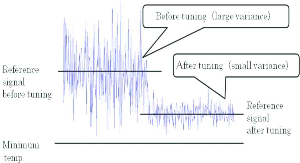
The example of the temperature control systems

These ways have the method based on the benchmark of the minimum variance control [4], the method to consider a fluctuation of the manipulated value as well as output error [5], the method to express the control performance to compare with data in the past in a plant concerned, and the way to limit the structure of the controller for example the a model based predictive control or PID control and express the control performance in the structure.

This research defines the good program makes the good control which realizes the small output variance.

3. MV-INDEX

This section introduces the calculation of MV-index which is proposed by Desborough and Harris [6].

The generalized controlled object described as the following Eq. (1).

where y(t) and d system output and minimum estimate value of dead time, respectively. u(t) is control input, and ξ(t) is probability noise including such as observation noise. In addition, when information about dead time cannot obtain anything, d is set as 1. Feedback control law is given as the following Eq. (2) for Eq. (1). where e(t) means the control error signal which is defined as [Eq. (3)]: From substituting (1) , (2) into (3) : Here, by considering the steady state, control error signal can obtain as the following Eq. (5). where the noise transfer function G_n(z⁻¹) can be divided the term about the dead time before and the term about the dead time after by the following Diophantine Eq. (6): where, G_n1(z⁻¹) is polynomial given by the following Eq. (7). From Eqs. (5) and (6) where G_d(z⁻¹) is defined as the following Eq. (9): And, Eq. (8) is expressed as the following Eq. (9) including Here, b(t) is not associated with the control input and if w(t – d) is possible to be 0 by the control input, let b(t) minimum variance output.

Here, σe2 shows the actual variance of control error and σMV2 shows achievable the minimum variance of control error at this system.

Furthermore, minimum-variance control performance assessment index η is shown by the following Eq. (11):

The range is 0 ≤ η ≤ 1 because σe2≥σMV2. The large value of MV-index η means that good control performance.

MV-index η can be calculated by Eq. (11). However, the numerator of Eq. (11) cannot be calculated directly. This term is obtained as the following procedure.

The following equation can be derived by multiplying z^−d for both sides of Eq. (10).

ξ(t – d) can be expressed from Eq. (12). The following Eq. (14) can be derived from Eqs. (8) and (14). Here, the following Eq. (15) is also obtained because the first term of Eq. (14) is same as b(t) of Eq. (11). Since the coefficient of the second term of Eq. (15) can be expressed as the finite transfer function, Eq. (16) can be expressed as the following AR model: The order p must be enough larger than the order of the controlled object. The relations of Eq. (16) are composed by the following matrix Eq. (17) of the form: where, e and X are constructed by previous signals. And, κ and b are the autoregressive parameter vector and modeling error vector, respectively.

These are expressed as [Eqs. (18)–(21)]:

where n is the sample length.

The parameters of Eq. (20) can be obtained by:

Therefore, the minimum variance can be obtained by Eq. (22).

4. SIMULATION EXAMPLE

This section demonstrates the effectiveness of the proposed scheme by a simulation example. The following Eq. (24) are used as the controlled object:

These models are discredited by 1.0 (s) sampling interval.

The following Eq. (25) is obtained as follows:

where the mean value of ξ is 0, ξ_σ = 0.05². The manipulate value u is limited as 0 < u < 100.

First, the ON–OFF control expressed as the following rule (26) was used for the controlled object (25).

This method is an example algorithm which is used by a beginner. This algorithm is conditional branch type which is studied on technology class in Junior high school.

Figure 2 is the control result by using the ON–OFF control. And MV-index is 0.0208 which calculated on 200 ≤ t ≤ 1200.

Figure 2

The result of the ON–OFF control

Next, the following PID control method (27) is used.

where k_p is the proportional gain, T_I is the reset time, T_D is the derivative time. Each value was set as k_p = 7.7, T_I = 17, T_D = 0.9, respectively. Figure 3 shows the control result by this PID control method. And MV-index is 0.2585 which is calculated on 200 ≤ t ≤ 1200.

Figure 3

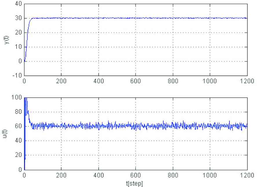
The result of the PID control

From the result of Figure 2, the input value is very oscillatory. The variance of the output value becomes large by the oscillatory input. From Figure 3, the variance of the output signal becomes small by the PID control. The MV-index can be the good metric to evaluate the programming performance.

5. CONCLUSION

This paper considers the using control performance assessment method for the achievement of the programming learning. In this paper, a method based on the controller performance assessment was proposed.

The effectiveness of the proposed method was evaluated by the simulation example.

ACKNOWLEDGMENT

This work was supported by JSPS KANKENHI (Grant Number 18K02980).

Author Introduction

Dr. Yoshihiro Ohnishi

He received his B.E. and M.E. from Okayama Prefectural University in 1997 and 1999, respectively. And he received his Dr. Eng. from Osaka Prefecture University in 2002. He is an associate professor at Faculty of Education in Ehime University. He is a member of SICE, ISCIE, IEEJ and IEEE.