
Time-Varying Lyapunov Function for Mechanical Systems
- DOI
- 10.2991/jrnal.k.190220.007How to use a DOI?
- Keywords
- Mechanical systems; time-varying systems; strict Lyapunov function; subsystems
- Abstract
In this paper, a general method for constructing time-varying Lyapunov functions is provided for mechanical systems. A new class of time-varying Lyapunov functions is provided and sufficient conditions of uniform asymptotical stability are established. Different from the existing results on this subject, we remove the periodic restrictions and persistency of excitation restrictions in our work. Moreover, the results are extended into the robustness cases with unmodeled dynamics. Based on the Lyapunov methods, it is shown that uniform asymptotical stability can be obtained by using the control input provided in our work.
- Copyright
- © 2019 The Authors. Published by Atlantis Press SARL.
- Open Access
- This is an open access article distributed under the CC BY-NC 4.0 license (http://creativecommons.org/licenses/by-nc/4.0/).
1. INTRODUCTION
In this paper, we investigate the stability problem of time-varying mechanical systems. It is well known that Lyapunov functions provide fundamental tools for stability analysis and controller design. In terms of Lyapunov functions, two research directions are widely investigated, that is, converse Lyapunov theory and constructions of Lyapunov functions. Converse Lyapunov theory guarantees the existence of smooth Lyapunov functions for some systems. However, construction methods give specific structures of Lyapunov function candidates. In this paper, we deal with the second research topic: construction methods. We aim to provide a generic approach for finding strict Lyapunov functions of nonlinear time-varying mechanical systems described by Euler–Lagrange equation. Several approaches for construction of strict Lyapunov functions have been proposed under various frameworks and control objectives [1,2].
In Han et al. [3], a new method for estimation the domain of attraction was shown by using non-strict Lyapunov functions. In Bretas and Alberto [4], an extension of invariance principle with non-strict Lyapunov functions was provided for power systems with transmission losses. In Hong et al. [5], strict Lyapunov functions were established for finite-time control problem of robot manipulators. In Zhang and Jia [6], two kinds of weak-invariance principles for nonlinear switched systems were developed and accurate convergent regions were obtained. The readers can refer to Malisoff and Mazenc [7], Mazenc [8], and Giesl and Hafstein [9] for more detailed discussions on this topic and a list of related references.
As we all know, some approaches have been well established to build explicit strict Lyapunov functions for time-invariant systems, such as variable gradient method, Krasovskii method and so on. But construction of strict Lyapunov functions for time-varying systems is a challenging problem and there are no general methods.
Motivated by the above considerations, we provide a general method for constructing time-varying Lyapunov functions of mechanical systems. We first consider a mechanical system with time-varying frictions. With the control input, the closed-loop system is obtained. Then, we divide the closed-loop system into two subsystems. For subsystem one, it is shown that the origin is uniformly asymptotically stable and a class of time-varying Lyapunov function V(t, x) is established. For the subsystem two, it is shown that the derivative of V(t, x) is bounded. Based on the derivatives of the time-varying Lyapunov function along the two different subsystems, we provide the time-varying Lyapunov function for the whole system. It is shown uniform asymptotical stability can be obtained with the control input provided in this paper.
2. PROBLEM STATEMENT
Consider the following mechanical system with time-varying friction [Equation (1)]
Property 1.
The matrix M is positive definite. Moreover, we define λmax as the maximum eigenvalue of M and λmin as the minimum eigenvalue of M.
Property 2.
The derivative of k(t) is bounded such that [Equation (2)]
Before presenting the main results, we give some lemmas first.
Lemma 1.
Zhang et al. [10] Let a,b,p,q be positive real numbers. If
Lemma 2.
Zhang et al. [10] Let ai > 0, bi > 0, i = 1,2, …, n, p > 1, and q > 1. If
Lemma 3.
Zhang et al. [10] For xi ∈ R, i = 1,2, …, n, and 0 < m < 1, then the following inequality holds [Equation (5)]:
Lemma 4.
For xi ∈ R, i = 1,2, …, n, and 0 < m < 1, then the following inequality holds [Equation (6)]:
Proof.
Let ai = |xi|m, bi = 1, i = 1, 2, …, n,
3. SUBSYSTEMS
For the uniform asymptotic stability problem of time-varying mechanical system (1), we propose the following control input [Equation (8)]
We define [Equation (10)]
Inspired by the results in Malisoff and Mazenc [7], we consider the following Lyapunov function [Equation (11)]
It can be verified directly that [Equation (12)]
The derivative of V(t, x) along subsystem
Similarly, the derivative of V(t, x) along subsystem
In the following, we define time-varying parameter
4. MAIN RESULTS
From (13) and (14), we can see that V(t, x) is not a Lyapunov function for system (1), because it is not easy to verify the negativity of the derivative of V(t, x) along system
Therefore, motivated by the results in Malisoff and Mazenc [7], we provide the following time-varying Lyapunov function [Equation (16) ]
Therefore, we conclude with the following theorem.
Theorem 1.
Consider time-varying system (1). If the control input is chosen as (8) with control parameters α and k0 large enough, then the closed loop system is uniformly asymptotically stable. Moreover, (16) is a strict Lyapunov function.
Proof.
This result can be verified by taking the derivative of V#(t, x) given in (16) directly. The detailed process is omitted here.
Then, we can extend the result to the robustness case. We take the following systems with unmodeled dynamics [Equation (18)]
Without detailed proof, we provide the following theorem for the robustness case.
5. NUMERICAL EXAMPLE
We give a numerical example to demonstrate the effectiveness of the proposed theoretical results under different initial values. Two different initial values are chosen as x(0) = (0.5, 0.3) and x(0) = (–0.1, 0.05), respectively. By using the control input (8), we can see that the state trajectories converge to the origin asymptotically (Fig. 1). The simulation clearly illustrate the exactness of our results.
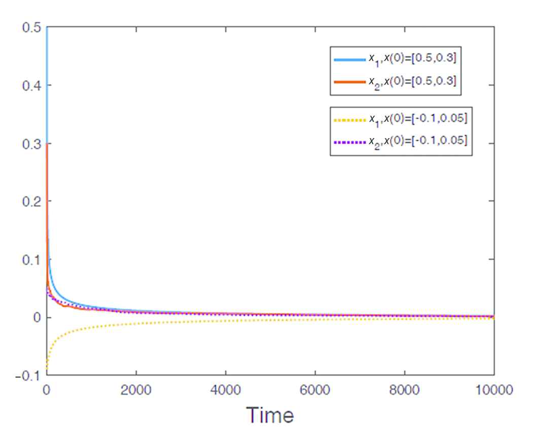
The state trajectories of system.
6. CONCLUSION
The stability problems have been considered in this paper for time-varying mechanical systems. A class of strict Lyapunov functions has been established, in which time-varying terms have been included. By using the new Lyapunov functions, concise criterion for uniform asymptotical stability have been provided. A numerical example has been presented for illustration.
ACKNOWLEDGMENT
This work is supported by the National Natural Science Foundation of China (Grant No. 61603050).
Authors Introduction
Dr. Bin Zhang
 He received his PhD degrees in control theory and applications from Beihang University, in 2016. He is with the School of Automation, Beijing University of Posts and Telecommunication. His research interests include multi-agent systems.
Dr. Yingmin Jia
 He received the B.S. degree in control theory from Shandong University, Jinan, China, in 1982, and the M.S. and PhD degrees in control theory and applications from Beihang University, Beijing, China, in 1990 and 1993, respectively. In 1993, he joined the Seventh Research Division, Beihang University, where he is currently a Professor of automatic control.
REFERENCES
Cite this article
TY  - JOUR
AU  - Bin Zhang
AU  - Yingmin Jia
PY  - 2019
DA  - 2019/03/30
TI  - Time-Varying Lyapunov Function for Mechanical Systems
JO  - Journal of Robotics, Networking and Artificial Life
SP  - 241
EP  - 244
VL  - 5
IS  - 4
SN  - 2352-6386
UR  - https://doi.org/10.2991/jrnal.k.190220.007
DO  - 10.2991/jrnal.k.190220.007
ID  - Zhang2019
ER  -