
Training Autoencoder using Three Different Reversed Color Models for Anomaly Detection
- DOI
- 10.2991/jrnal.k.200512.008How to use a DOI?
- Keywords
- Convolutional neural network; autoencoder; anomaly detection; color models
- Abstract
Autoencoders (AEs) have been applied in several applications such as anomaly detectors and object recognition systems. However, although the recent neural networks have relatively high accuracy but sometimes false detection may occur. This paper introduces AE as an anomaly detector. The proposed AE is trained using both normal and anomalous data based on convolutional neural network with three different color models Hue Saturation Value (HSV), Red Green Blue (RGB), and our own model (TUV). As a result, the trained AE reconstruct the normal images without change, whereas the anomalous image would be reconstructed reversely. The training and testing of the AE in case of RGB, HSV, and TUV color models were demonstrated and Cifar-10 dataset had been used for the evaluation process. It can be noticed that HSV color model has been more effective and achievable as an anomaly detector rather than other color models based on Z- and F-test analyses.
- Copyright
- © 2020 The Authors. Published by Atlantis Press SARL.
- Open Access
- This is an open access article distributed under the CC BY-NC 4.0 license (http://creativecommons.org/licenses/by-nc/4.0/).
1. INTRODUCTION
The Artificial Intelligence (AI) is widely used and has been existed over many decades. It uses the information originating from sensors, images, languages and texts. Analyzing this information giving hypothesis leading to make decision [1]. AI can be viewed as a set that contains Machine Learning (ML) and Deep Learning (DL) [2]. DL is often categorized as supervised or unsupervised [3]. Autoencoders (AEs) are one of the DL methods which trained in an unsupervised fashion to automatically extract features of training data [4]. Moreover, anomaly detection is one of the most important applications of AEs [5]. One of the training methods that has been used for anomaly detection is a Convolutional Neural Network (CNN). CNN has been applied in various modern applications, and it is often implemented in image analysis [6], speech and face recognition [7] and autoencoders [8] with great success.
The aim of this study is to use CNN-autoencoder trained with three different color models; Hue Saturation Value (HSV), Red Green Blue (RGB) and our own model (TUV) to improve the detection accuracy especially the anomalous one.
2. RESEARCH CONCEPT
The main concept focuses over using the autoencoder trained with reversed color models in order to detect the anomaly data.
2.1. Autoencoder
Autoencoders are neural networks that aims to copy their inputs to their outputs. It is used to automatically extract features of training data. AEs are applied for object recognition systems that being used the anomaly detectors [5]. To improve a recognition accuracy, the anomaly detectors has the ability to remove anomalous objects before recognition process to reduce misrecognition. AEs are composed of three fully connected layers: input, hidden, and output layers. These layers are trained to reconstruct input data on the output layer as shown in Figure 1.
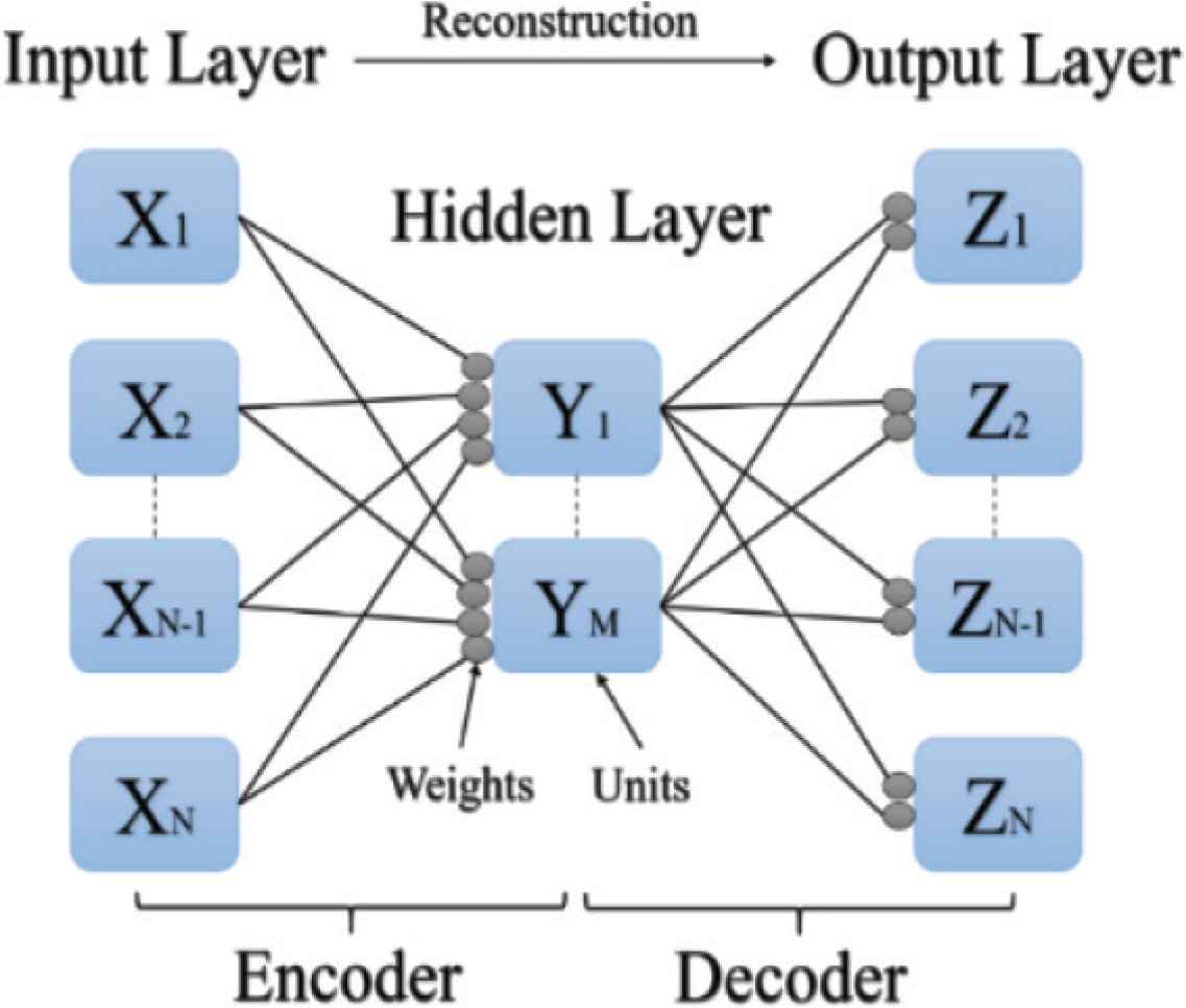
Structure of autoencoder.
2.2. Anomaly Detection
The idea in anomaly detection based on machine learning, is to model the normal behavior of data in the training period, and then try to fit the test data using the trained model. In case a large inconsistency is found between the fitted model and the trained model, the test data is regarded as anomalous.
When using autoencoders, which applies dimensionality reduction to the input data, for anomaly detection, we assume that the data contains variables that can be represented in lower dimensions. These variables are also assumed to be correlated with each other and would show significant difference between normal and anomalous samples [9].
There are two types of training data for autoencoder to detect anomaly images; labeled and unlabeled data. Based on the type of data, the anomaly detection algorithm differs. In case of labeled data, conditional distributions can distinguish between correct and anomalous data. Accordingly, the probability of the conditional distribution determines whether the data is correct or anomalous. On the other hand, a generative model trained with correct data is used as a detector for unlabeled data. The inability of the model to generate a correct output for anomalous data is utilized to detect anomaly.
3. METHODOLOGY
The autoencoder reconstruct the input to the output even if the input was an anomalous data, and the Mean Square Error (MSE) between input and output will be small in case of normal or an anomalous input, and the detection will be difficult especially for the anomalous one. Our goal is to maximize the difference of reconstruction error by reconstructing the anomaly classes reversely. Therefore, the MSE will be bigger and the anomaly detection will be easier as shown in Figure 2.
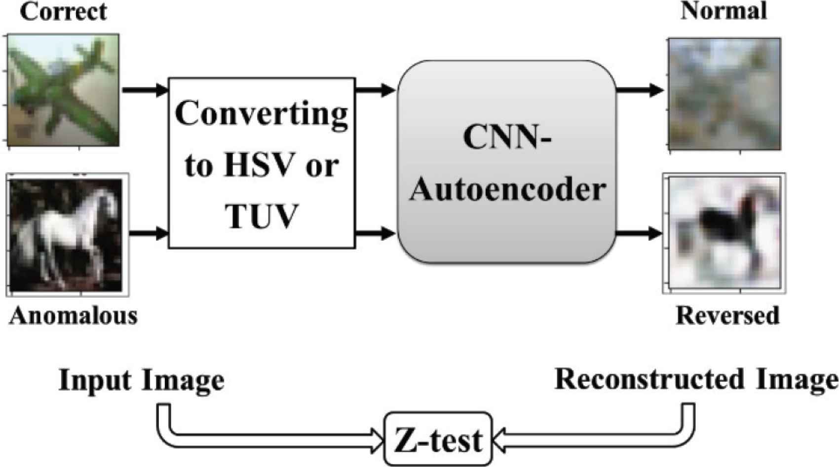
Block diagram of training method.
3.1. Detection Algorithm
The first step of the algorithm is to convert the training dataset images from RGB color model to HSV [10] or TUV as shown in Figure 3a and 3b respectively. Using the Equations (1)–(3) for HSV color model, and Equations (4)–(6) for TUV color model.
Hue calculation (H):
Saturation calculation (S):
Value calculation (V):
R′ = R/255, G′ = G/255, B′ = B/255.
Cmax = max (R′, G′, B′), Cmin = min (R′, G′, B′), and Δ = Cmax − Cmin
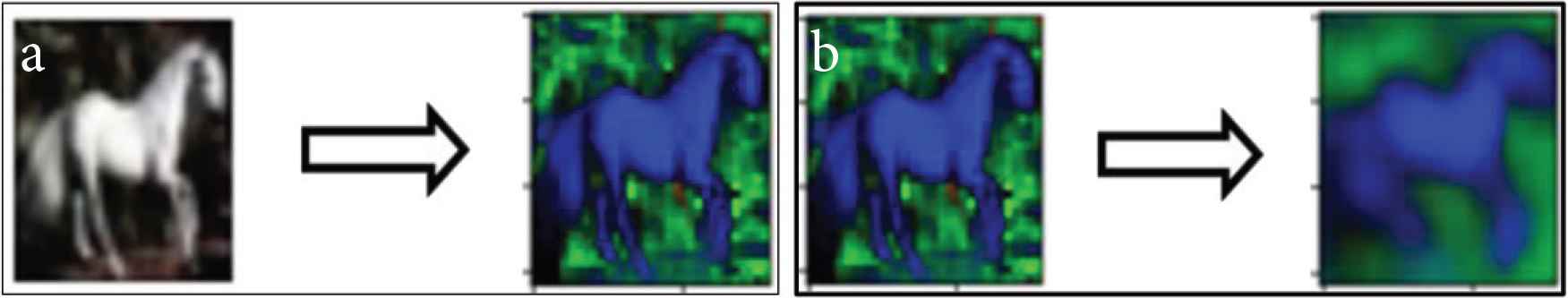
Converting training dataset images, (a) RGB to HSV, (b) HSV to TUV.
Notice in the case of HSV color model the value range for hue, saturation and value are 0–179, 0–255 and 0–255 respectively.
Secondly, the anomalous data is reversed as a result of the next step as shown in Figure 4, using the following Equations (7)–(9),
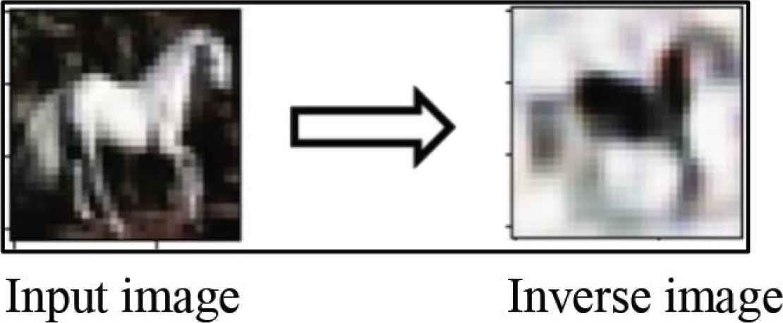
Inversing the anomalous image.
Consequently, the AE is trained using the new training dataset based on CNN. The proposed training patterns for AE are as follows: (1) the first case the autoencoder is trained by class 0 as normal and other classes as anomalous, (2) the second case the classes 0 and 1 will be normal and other classes are reversed. Consequently, the number of normal classes will increase for each next case. Finally the autoencoder will be trained with all classes as normal for the last case. Final step of the algorithm is to evaluate the performance of the AE using an inference dataset. Figure 5 illustrates the structure of CNN-autoencoder. As shown in the figure, the input image with size 32 × 32 × 3 is firstly convoluted in the first layer by a 5 × 5 filter.
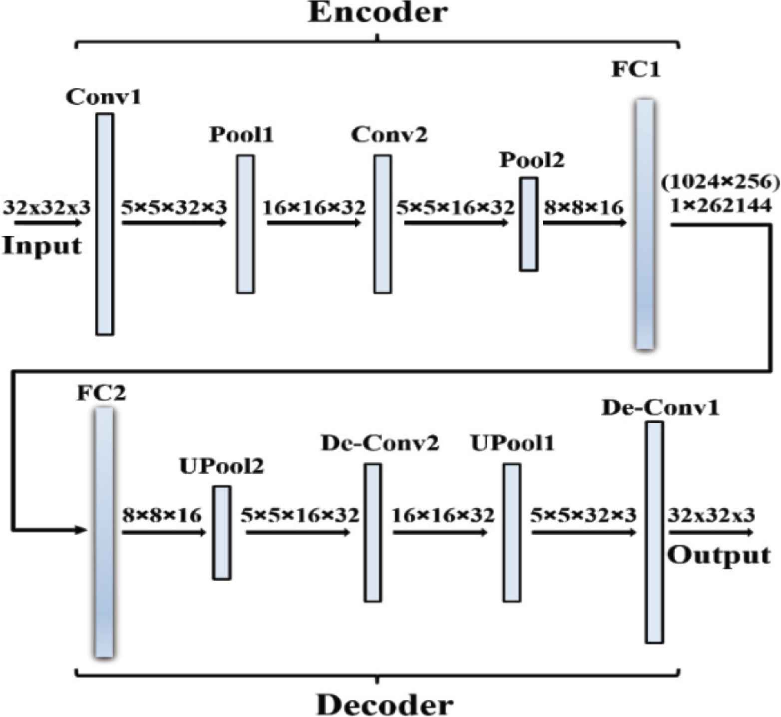
Structure of convolutional neural network autoencoder.
Consequently, the image dimensions are reduced through a pooling layer from size 5 × 5 × 32 × 3 to size 16 × 16 × 32. Next, another convolution layer is applied followed by a pooling layer to change the size of the image from 5 × 5 × 16 × 32 to 8 × 8 × 16. Finally, the encoding process is finalized with a fully connected layer with the output size of 1 × 262144 (1024 × 256). In order to decode the image, the reverse of the previous process is applied and finally a reconstructed image with the same dimensions as the input image is the same as the output.
3.2. Cifar-10 Dataset
The CIFAR-10 dataset is a set of images that can be used to teach a computer how to recognize objects, it contains RGB images with 32 × 32 pixels’ size. It has 10 classes and each class contains a different type of images. The dataset divides into a 50,000 images training set and 10,000 images testing set. Each set has an equal distribution of elements from each one of the 10 classes [11], as shown in Table 1.
| Normal labels | The number of images depending on training patterns | The number of images depending on test patterns | ||
|---|---|---|---|---|
| Normal | Anomalous | Normal | Anomalous | |
| 0 | 5000 | 45,000 | 1000 | 9000 |
| 0 and 1 | 10,000 | 40,000 | 2000 | 8000 |
| 0–2 | 15,000 | 35,000 | 3000 | 7000 |
| 0–3 | 20,000 | 30,000 | 4000 | 6000 |
| 0–4 | 25,000 | 25,000 | 5000 | 5000 |
| 0–5 | 30,000 | 20,000 | 6000 | 4000 |
| 0–6 | 35,000 | 15,000 | 7000 | 3000 |
| 0–7 | 40,000 | 10,000 | 8000 | 2000 |
| 0–8 | 45,000 | 5000 | 9000 | 1000 |
| 0–9 | 50,000 | 0 | 10,000 | 0 |
The number of images depending on training and testing patterns
3.3. Evaluation of Performance for Autoencoder
For significance validation, both F- and Z-test were conducted. The Z-score value can be calculated based on the following formula (10) [12]:
A p-value is used in hypothesis testing to help accepting or reject the null hypothesis. It is evidence against a null hypothesis. The smaller the p-value, the stronger the evidence that you should reject the null hypothesis.
The used hypothesizes are; if p-value >0.05, then there is no significant difference between the input and reconstructed image (i.e. considered as Normal).
If p-value <0.05, then there is significant difference between the input and reconstructed image (i.e. considered as Anomaly).
4. RESULTS AND DISCUSSION
4.1. Training and Testing Loss
The difference between the test data input images and the reconstructed images were calculated in each epoch. The relationship between the testing loss and the epochs is shown in Figure 6. It is worth mentioning that the value of the test loss is almost similar or close to train loss value and this indicates to a good reconstruction process.
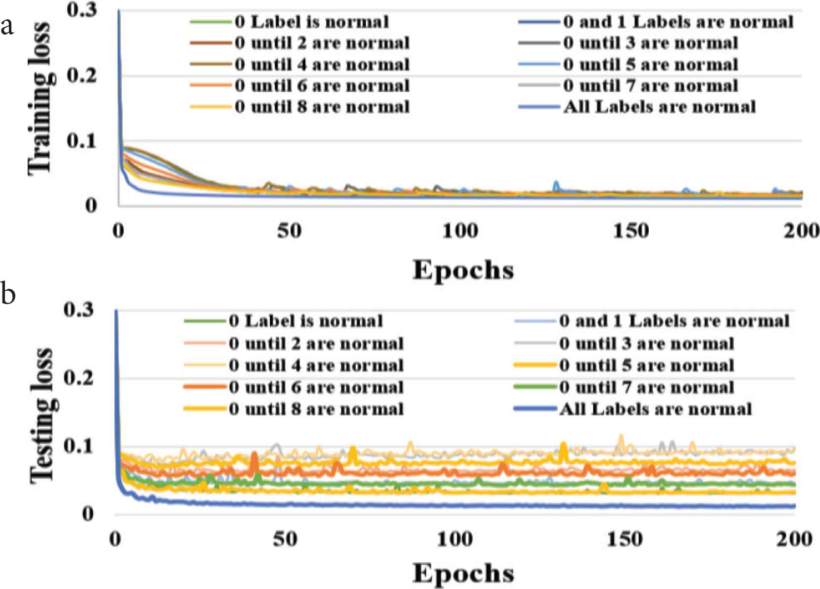
Training and testing loss against epochs for HSV color model, (a) training loss, (b) testing loss.
4.2. Z-test
The p-value of each color model was calculated at zero mean value for each class and the results were shown in Tables 2–4 for the three cases; in the first one only class 0 is normal while the rest are anomaly, in the second case classes 0–7 are normal and other classes are anomaly, and in the last one all classes are normal. From Table 2, it is clear that HSV in class 0 is better than RGB and TUV as the p-value is 0.5819 which is larger than 0.2013 and 0.2941. This is because in the normal class the difference between input and output image should be small as proven by p-value result. In contrast, most of p-values of anomaly classes in RGB and TUV are bigger than in HSV which denotes the HSV detects the anomaly classes more effectively than other color models. Similarly, Tables 3 and 4 show that, generally, HSV in all classes is better than RGB and TUV as the detection in HSV is more achievable than other models.
| Classes | Color model type | ||
|---|---|---|---|
| HSV | RGB | TUV | |
| 0 | 0.5819 | 0.2013 | 0.2941 |
| 1 | 0.0057 | 0.0298 | 0.0012 |
| 2 | 0.0000 | 0.0100 | 0.0084 |
| 3 | 0.0076 | 0.0008 | 0.0142 |
| 4 | 0.0000 | 0.0222 | 0.0010 |
| 5 | 0.0005 | 0.0182 | 0.0109 |
| 6 | 0.0053 | 0.0322 | 0.0103 |
| 7 | 0.0213 | 0.0178 | 0.0478 |
| 8 | 0.0166 | 0.0424 | 0.0000 |
| 9 | 0.0267 | 0.0323 | 0.0377 |
p-value for class 0 as normal and classes 1–9 as anomalous hypothesis for HSV, RGB and TUV
| Classes | Color model type | ||
|---|---|---|---|
| HSV | RGB | TUV | |
| 0 | 0.9473 | 0.7742 | 0.1296 |
| 1 | 0.7223 | 0.1920 | 0.6506 |
| 2 | 0.9847 | 0.1795 | 0.3149 |
| 3 | 0.0760 | 0.6836 | 0.1061 |
| 4 | 0.4545 | 0.1688 | 0.5228 |
| 5 | 0.5675 | 0.9366 | 0.1699 |
| 6 | 0.0882 | 0.4278 | 0.8637 |
| 7 | 0.4240 | 0.2964 | 0.2785 |
| 8 | 0.0041 | 0.0000 | 0.0000 |
| 9 | 0.0012 | 0.0003 | 0.0000 |
p-value for classes 0–7 as normal and classes 8 and 9 as anomalous hypothesis for HSV, RGB and TUV
| Classes | Color model type | ||
|---|---|---|---|
| HSV | RGB | TUV | |
| 0 | 0.4440 | 0.1899 | 0.1262 |
| 1 | 0.8405 | 0.6838 | 0.1086 |
| 2 | 0.6534 | 0.7221 | 0.0653 |
| 3 | 0.7256 | 0.8480 | 0.0853 |
| 4 | 0.3155 | 0.1685 | 0.0645 |
| 5 | 0.5290 | 0.1529 | 0.0792 |
| 6 | 0.8100 | 0.5489 | 0.0635 |
| 7 | 0.1732 | 0.4731 | 0.4457 |
| 8 | 0.5756 | 0.3557 | 0.2570 |
| 9 | 0.8039 | 0.8849 | 0.0792 |
p-value for classes 0–9 as normal hypothesis for HSV, RGB and TUV color models
4.3. F-test
An anomaly detection performance is usually evaluating by using the F-test using the recall and precision as shown in Equation (11) [14]. Accomplishing high recall and high precision is not easy at the same time because the recall and precision goals are often conflicting.
Figure 7 shows the F-test against the threshold for HSV, RGB and TUV respectively. The first mean point in comparing with the previous work is the horizontal range for the F-test. This range in the proposed method was small, therefore, the correct threshold for the detection could be defined easily. The second point is that F-value in the previous work was bigger in case of RGB than the value in our proposed method and that indicates increasing in the accuracy. In proposed method, the F-test for HSV color model is better than other models.
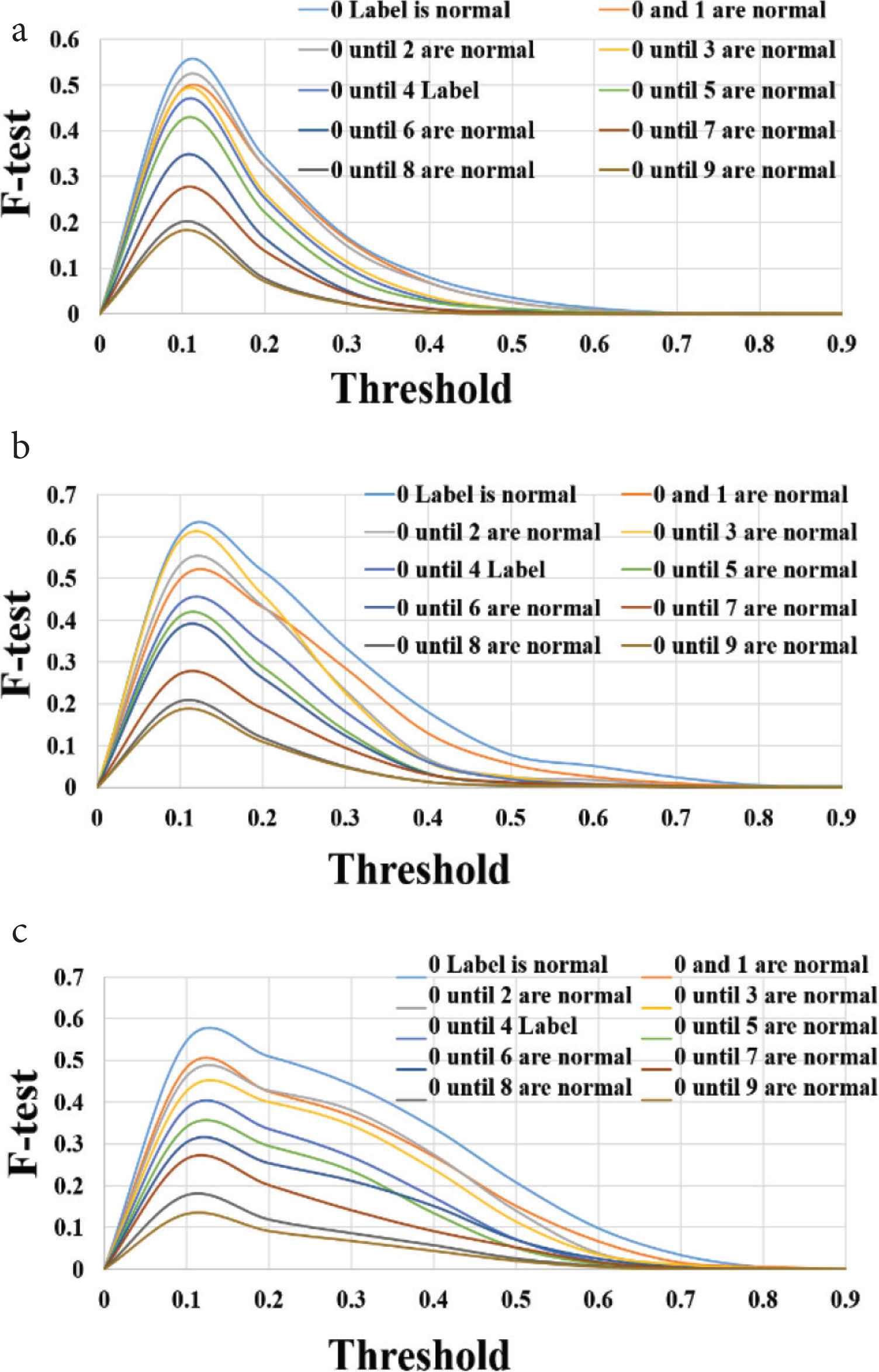
(a) F-test for RGB, (b) F-test for HSV, (c) F-test for TUV.
Table 5 represents the comparison between our results and the previous results, the proposed CNN-autoencoder has been trained with three different color models HSV, RGB and TUV, whereas the stacked autoencoder trained with one color model which is RGB. Besides, the reconstruction quality results using the proposed CNN-autoencoder for the same color model (RGB) were better than the reconstruction results using the stacked autoencoder in spite of using the same dataset for the evaluation process.
| Previous method [13] | Proposed method | ||
|---|---|---|---|
| Training color model | RGB | RGB, HSV and TUV | |
| Structure | Stacked AE | CNN-AE | |
| Dataset | Cifar-10 | Cifar-10 | |
| Reconstruction quality | • RGB | Moderate | Good |
| • HSV | NA | Good | |
| • TUV | NA | Moderate | |
| F-test | • RGB | Good | Moderate |
| • HSV | NA | Good | |
| • TUV | NA | Moderate | |
| Z-test | • RGB | NA | Moderate |
| • HSV | NA | Good | |
| • TUV | NA | low | |
General comparison between previous and proposed methods
5. CONCLUSION
This research investigates the anomaly detection using CNN-autoencoder trained with three different color models. The trained AE has reconstructed the correct input normally, whereas the anomalous input has been reconstructed reversely. The results at 200 epochs training show that HSV color model has been more effective in anomaly detection rather than other models based on Z- and F-test analyses.
CONFLICTS OF INTEREST
The authors declare they have no conflicts of interest.
ACKNOWLEDGMENT
This research was supported by JSPS KAKENHI Grant Numbers 17K20010.
AUTHORS INTRODUCTION
Mr. Obada Al aama
 He graduated from Al-Baath University Department of Communication and Electronics Engineering, Syria, in 2013. He received Master of Engineering degree from Kyushu Institute of Technology, Japan, in 2019. His research interests include image processing, deep learning and neural networks.
Associate Prof. Hakaru Tamukoh
 He received the B.Eng. degree from Miyazaki University, Japan, in 2001. He received the M.Eng. and the PhD degree from Kyushu Institute of Technology, Japan, in 2003 and 2006, respectively. He was a postdoctoral research fellow of 21st century center of excellent program at Kyushu Institute of Technology, from April 2006 to September 2007. He was an Assistant Professor of Tokyo University of Agriculture and Technology, from October 2007 to January 2013. He is currently an Associate Professor in the Graduate School of Life Science and System Engineering, Kyushu Institute of Technology, Japan. His research interest includes hardware/software complex system, digital hardware design, neural networks, soft-computing and home service robots. He is a member of IEICE, SOFT, JNNS, IEEE, JSAI and RSJ.
REFERENCES
Cite this article
TY  - JOUR
AU  - Obada Al aama
AU  - Hakaru Tamukoh
PY  - 2020
DA  - 2020/05/20
TI  - Training Autoencoder using Three Different Reversed Color Models for Anomaly Detection
JO  - Journal of Robotics, Networking and Artificial Life
SP  - 35
EP  - 40
VL  - 7
IS  - 1
SN  - 2352-6386
UR  - https://doi.org/10.2991/jrnal.k.200512.008
DO  - 10.2991/jrnal.k.200512.008
ID  - Alaama2020
ER  -