
Verification of a Combination of Gestures Accurately Recognized by Myo using Learning Curves
- DOI
- 10.2991/jrnal.k.200512.009How to use a DOI?
- Keywords
- Learning curve; data distribution; Myo armband; American sign; reliable gesture recognition
- Abstract
This paper studies verification of a combination of hand gestures recognized by using the Myo armband as an input device. To this end, relationship between data distribution and learning curves is investigated for binary classification and multi-class classification problems. A verification method is then proposed for finding a combination of gestures accurately classified. Experiments show effectiveness of the proposed method.
- Copyright
- © 2020 The Authors. Published by Atlantis Press SARL.
- Open Access
- This is an open access article distributed under the CC BY-NC 4.0 license (http://creativecommons.org/licenses/by-nc/4.0/).
1. INTRODUCTION
A technique for hand gestures recognition from surface ElectroMyoGraphy (sEMG) is useful for extending means of human communication. To find the rule of sEMG that corresponds to the state of hand gestures, machine learning is often used (e.g. Savur and Sahin [1] and Galea and Smeaton [2]). Recently, the Myo armband [3] is one of the most popular sEMG acquisition systems, because it is relatively inexpensive and easy to remove. The Myo armband is being regarded as one of the tools for operating virtual reality (VR) [4] and for communicating with hearing impairment [1], and so on.
In developing various applications of Myo as an input device, it is important to verify a combination of gestures learned from the Myo data, because we cannot develop a reliable application without finding a combination of gestures accurately classified. To find such a combination, we need to confirm that the number of the data used for learning is sufficient, but we cannot from a single matrix of classification accuracy.
There is a method for confirming that the number of the data used for learning is sufficient; that is using a learning curve [5]. The meaning of the learning curve in the context of machine learning is mainly divided into two [6]. One is a graph that is created by plotting performance measure against the training iteration on the condition that the number of training data is fixed. The other is a graph that is created by plotting performance measure against the number of the data used for training. In this study, we mean the learning curve by the second graph; it is created by plotting classification accuracy of training or test against the number of data for training.
In several studies, the learning curve has been used for predicting the data required for DNA classification [7] and for comparing the methods of machine learning algorithms [8], and so on. These studies have used the averaged learning curve, which is an average of the discrimination accuracy of all classes. In contrast, Wahba et al. [9] proposed to use the learning curve for individual classes.
Learning curves are useful for verifying a combination of gestures accurately classified, because they possibly offer information on the boundary and data distributions. Learning curves indeed indicate accuracy of a classifier, and accuracy depends on the boundary and data distributions. However, the relationship between learning curves and data distributions has not been clear. If the relationship is clarified, it would be useful for inferring them in a high dimensional space.
There are a lot of studies on gesture recognition using the Myo armband [1,2,10]. But research has not been done for finding a combination of gestures accurately classified in the light of learning curves.
In this paper, we study relations between learning curves and data distribution. We then verify a combination of gestures accurately classified using a Myo armband.
2. MYO ARMBAND AND GESTURES
Myo (Figure 1) is an armband type gesture controller developed by Thalmic Labs. It measures sEMG of the arm (Figure 2). Myo has sEMG sensors of eight channels and its sampling frequency is 200 Hz. The sEMG measured by each channel is converted from analog to digital and is sent to the PC as an integer value between −128 and 128 by Bluetooth. The signal indicates the amount of active muscle fibers and is a dimensionless value.
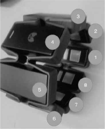
Myo armband it has eight channels.
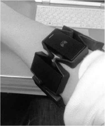
Wearing Myo armband.
Let us represent the sEMG by v|(t), where l is the number of channel (| = 1, …, 8) and t is the time index (t = 1, …, Nv). We use the average of the absolute value w|(t) for each channel in 1 s as features for classification and define as follows:
American Sign Language (ASL) is a sign language mainly used in North America. It is published by National Institute on Deafness and Other Communication Disorders [12] and shown in Figure 3. We deal with the sEMG data of 24 gestures except “j” and “z” in ASL, because we classify the hand gestures by using only the sEMG data and the gestures of “j” and “z” include motion of fingers. To conduct experiments, we make training and test dataset. The size of each dataset is 24 × 100. We use K-nearest neighbor of the scikit-learn toolkit for classification.
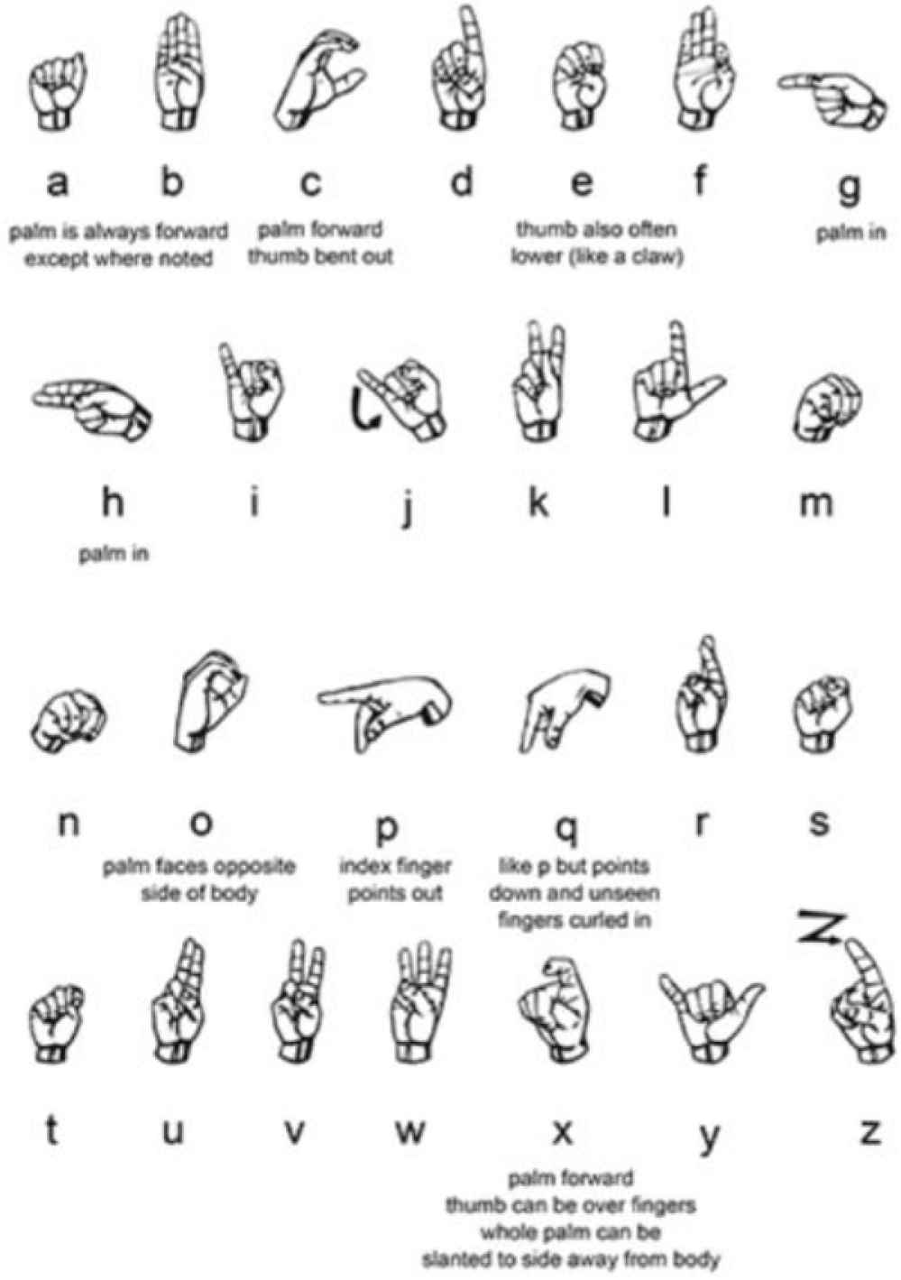
American sign language [12].
3. LEARNING CURVE AND DATA DISTRIBUTION
In this section, given the training and test data sets, we study characteristics of learning curves. We first consider a binary classification problem given the uniformly distributed data, and then a multi-class one given the normally distributed data. Suppose that the training data
We construct the learning curve by increasing the training data one-by-one chosen from the given data. We compute the learning curve by taking the average, because the learning curve depends on how to increase the training data. We will show how to increase the data in Appendix A.
3.1. Binary Classification Problem
Suppose that the dimension f of the feature space is 1 and consider a binary classification problem (c = 2). Assume that the training data belonging to A and B are given and are uniformly distributed as follows:
We show the distribution of training and test data in Figure 4. The classification boundary is 0.55, if the number of the training data is sufficiently large, because the boundary is between 0.5 and 0.6 in the training data set and the boundary 0.55 maximizes the margin of classification. If the number of training and test data, N and M, are sufficiently large, the percentage of the blue area in Figure 4 represents the misclassification rate:
The misclassification rate e is obtained by the volume of the misclassification areas of A′ and B′ (blue areas), supposing that the data of A′ and B′ are uniformly distributed. The accuracy rate is moreover given by 1 − e for large M and N.
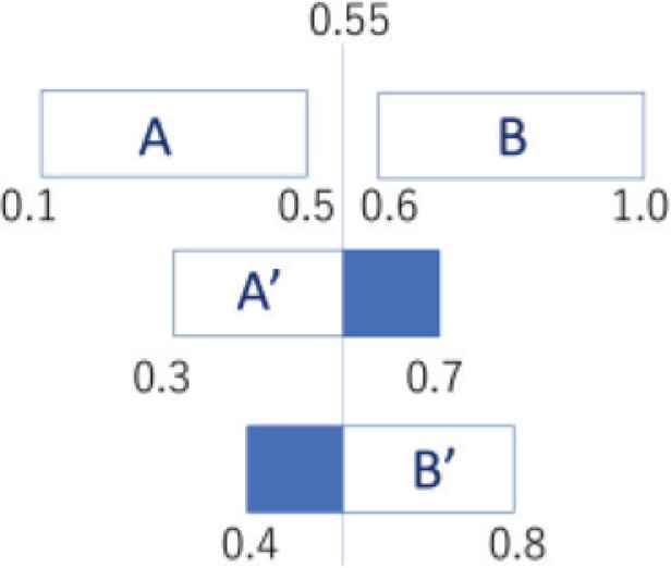
The distribution of training and test data. The first row represents the training data, and the second and third rows the test data. The data in the blue area is misclassified by the classification boundary 0.55.
The learning curve is created by plotting the classification accuracy 1 − ei against the number of training data i, where ei is misclassification rate for i. The accuracy of the learning curve 1 − eN approaches 1 − e, as the number of the training data N becomes large. We therefore see that the accuracy rate 1 − e of the classification for the test data (Figure 4) is related with that for sufficiently large data in the learning curve (Figure 5). This fact implies that the accuracy rate of K-nearest neighbor is 1 − 0.375 (62.5%), if N and M are sufficiently large.
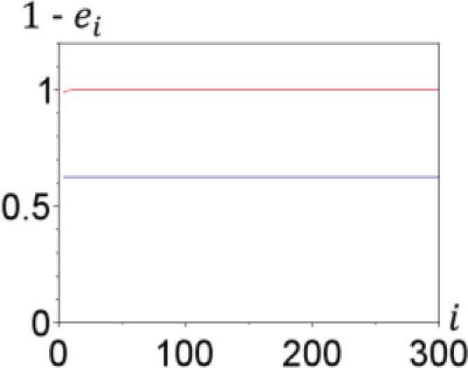
Learning curves. Blue and red curves respectively represent the learning curves for the training and test data. The value of the learning curve for the test data at i = 300 is approximately 62.5%.
Let us consider the case where N and M are finite. We draw the learning curves of training and test data by averaging m learning curves obtained by the m maps (SN,k); see Appendix A. We use p as an identifier (p = 1,…,m). We describe the number of the test data for p as M(p) and suppose that the classifier sets a classification boundary at z(N), given N training data. We express the total numbers of k satisfying the following inequalities respectively by MA′(p) and
In the same way, we express the total numbers of k satisfying the following inequalities respectively by MB′(p) and
The accuracy rate 1 − eN is then given by averaging the accuracy calculated from the number of correctly classified data (Appendix A):
The left hand side of (2) is related to the learning curve at N, and the right hand side depends on the test data and the boundary set by the N training data. In other words, the right hand side represents the percentage of data that does not violate the boundary. It should be noted that the test data are uniformly distributed, but the right hand side of (2) can be calculated regardless of the distribution, by just counting the number of not violating the boundary.
3.2. Multi-class Classification Problem
We study a multi-class classification problem. Let us consider data in feature space of f = 2 dimensions and classify them into c = 3 classes. Suppose that normally distributed data wA(n), wB(n), and
Assume that normally distributed data wA′(n), wB′(n), and
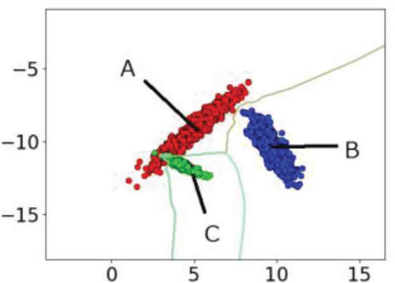
Training data indicating three classes of A, B and C. The green line is the boundary of the classes.
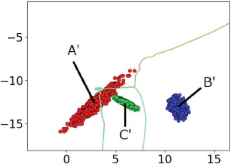
Test data indicating three classes of A′, B′ and C′. The green line is the boundary of the classes.
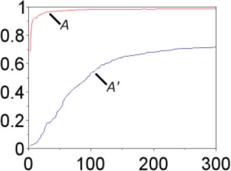
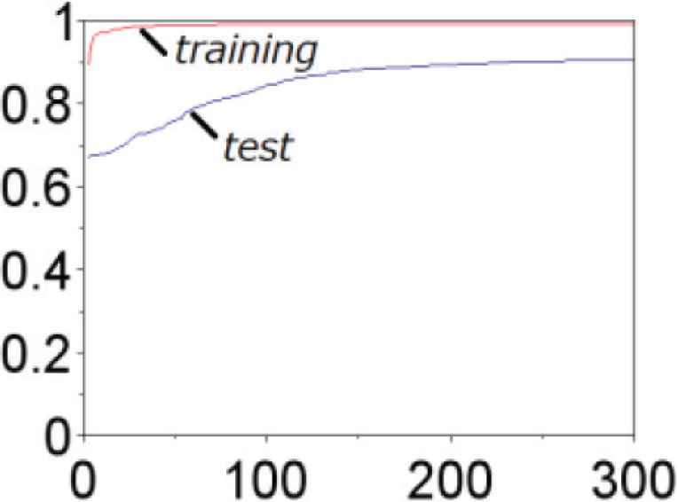
Learning curves (A, A′). Red line is the learning curve of training, and blue line is that of test.

Learning curves (B, B′). Red line is the learning curve of training, and blue line is that of test.
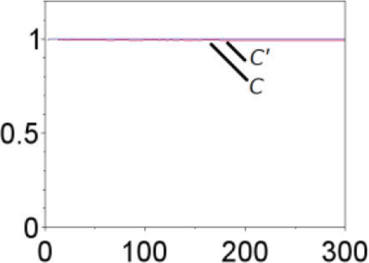
Learning curves (C, C′). Red line is the learning curve of training, and blue line is that of test.
Learning curves (averaged). Red line is the learning curve of training, and blue line is that of test.
From the individual learning curves of training and test data in Figures 8–10, we examine the relationship between the classification boundary and the distribution of the training and test data in Figures 6 and 7.
In the same way as deriving (2), we see that the accuracy of the test data B′ is equal to the ratio of the data B′ that does not violate the boundary determined by the training data A, B and C. The label B′ is indeed classified with 100% accuracy as shown in Figure 9, indicating that all test data of B′ are not outside of the trained area of B (Figure 7). The label B is also classified with 100% accuracy (Figure 9), showing that all training data of B can be trained correctly (Figure 6). We observe that the labels C and C′ are also classified with almost 100% accuracy. On the other hand, we see from the learning curve in Figure 8 that accuracy of classification of A′ at 300 sets of data is about 70%. This fact implies that the test data of A′ cross the classification boundary and that some of them are outside of the classification area of A as shown in Figure 7.
We can obtain the ratio of misclassification caused by changes of distribution between training and test, from the gap between the learning curves of training and test data. For example, there is a gap between A and A′ in Figure 8. In this case, the ratio of test data correctly classified is lower than that of training data. This is because the test data A′ violates the boundary defined by the training data A in Figure 7. On the other hand, the data B′ is correctly classified by the boundary set by the training data. In this way, we can find test data seriously affected by distribution changes, by constructing individual learning curves.
4. EXPERIMENTS
We investigate characteristics of the data of Myo in Section 4.1 and propose a method for finding a combination of gestures accurately classified in Section 4.2.
Let us consider data in a feature space of f = 8 dimensions and classify them into c = 24 classes; they corresponds to characters of the alphabet except “j” and “z”. Using wl(j) in (1), we define the data of Myo in the feature space as
4.1. Visualization of Myo Data
We visualize the features extracted from the data of Myo to see the characteristics of the data distribution. Figures 12 and 13 indicate the results of principal component analysis showing eight-dimensional feature values obtained from Myo by reducing the dimensions to 2. Each of the three classes corresponds to a, b, and f gestures. Even if Myo is not removed between training data acquisition and test data acquisition, the data distribution changes between training and test data acquisition, and it makes learning difficult. This is true for the case where Myo is removed as well. We will therefore study verification of a combination of gestures using learning curves based on the investigation of the boundary and the test data in Section 3.
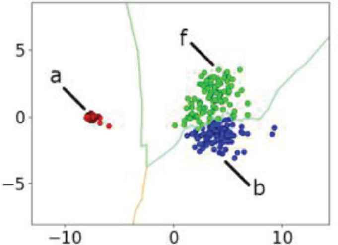
Training data of Myo.
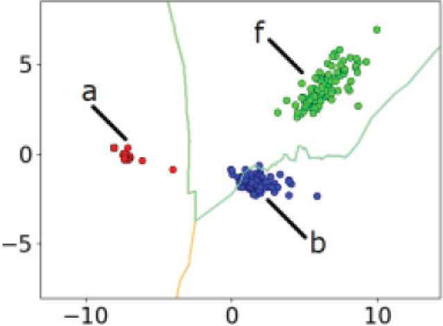
Test data of Myo.
4.2. Method for Verification
We verify a combination of gestures that can be classified with high accuracy. We first acquire 24 training and test data labeled “a” to “y” except “j”. We then make verification, using individual learning curves and averaged ones and conducting experiments for acquiring data.
Suppose that the numbers of training and test data are the same (N = M). Let us draw individual learning curves of training and test data. If accuracy is low for a label (e.g. “k”) in both training and test data at N and if the gap between them are very small, then there is a possibility that accuracy of the classifier for the label (e.g. “k”) may be enhanced by excluding another label that makes conflict for classification. We should therefore keep such a label (e.g. “k”), if the gap between learning curves of training and test data is small. On the other hand, if there is a large gap between the training and test data in learning curves of a label (e.g. “f”), then the label (e.g. “f”) should be excluded from the classification target.
We show an example of learning curves for a gesture to be excluded in Figure 14. Even if the learning curve of training is seen that classification is possible, the gesture should be excluded from the classification target in case that the learning curve of test data at N indicates low accuracy because of the gap between the training and test data. We show another example of the gesture regarded as a classification target in Figure 15. Accuracy for training and test data are both high, and there is almost no gap between them.
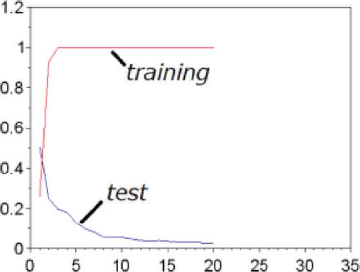
Example of learning curves for a gesture (“f”) to be excluded.
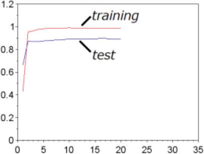
Example of learning curves for a gesture (“k”) not to be excluded.
Let us reduce the number of the combination of gestures from cs to ce for finding a reliable one. Based on the above consideration, the combination of gestures is verified by the following verification algorithm.
[Verification algorithm]:
Step 1: Draw individual learning curves and an averaged one for the number of classes cs.
Step 2: Exclude the gesture that has a large gap between learning curves of the training and test data. If there are no more gestures to be excluded, then go to Step 5.
Step 3: Re-acquire data for gestures that are not excluded in Step 2 and draw the individual and averaged learning curves.
Step 4: Repeat Steps 2 and 3 until there are no more gestures that can be excluded in Step 2.
Step 5: Re-acquire data for not excluded gestures and draw the individual and averaged learning curves. Check if an averaged learning curve has a satisfactory discrimination accuracy. If it is unsatisfied, go to Step 2.
In Step 2, excluded gestures are determined by referring the accuracy indicated by the learning curve as shown in Figures 14 and 15. Suppose that the number of the training data is α. In this experiment, α is 20. The value of α depends on the user who allows how much time for learning. The more α is increased, the more time is needed for learning. Of course, the user can reduce the value of α by seeing the learning curve.
We make experiments and apply the proposed method to the data. Since data distribution depends on removal of Myo between experiments, we investigate verification by taking the interval time between test and training data acquisition into account. We thus consider two cases: For the first case we do not remove Myo between data acquisition (Case 1), and for the second case we do it. We moreover consider two cases in the second case: There is little time in the interval (Case 2), and there are several days (Case 3). We apply the verification algorithm and conduct experiments in the order of Cases 1–3, since the number of the reliable combination is decreased in the order of them.
4.3. Results of Experiments
We determined the threshold γ for the gap of accuracy between training and test data as 20%. We obtained a combination of gestures with high accuracy for each of Cases 1–3, extracting a combination of gestures that was not in a trade-off relationship. As a result, we found the followings. In Case 1, five gestures “e”, “k”, “q”, “r”, and “y” can be classified with 100% accuracy. Also, in Case 2, the classifier obtained by the verification algorithm can classify the four gestures “e”, “k”, “q”, and “y” with 99% accuracy. But in Case 3, only two gestures “k” and “q” are classified with 99% accuracy.
5. CONCLUSION
In this study, we investigated the relationship between data distribution and learning curves, and we then verified a combination of ASL that is accurately classified using a Myo armband. In addition, as a result of investigating the characteristics of the data acquired from Myo, it was found that the distribution of data changes between the interval of training and test data acquisition, and verifications were hence carried out for the cases of different intervals. It remains a future topic how to determine the threshold γ for the gap to ensure accuracy.
APPENDIX A. APPENDICES
Suppose that the data
We explain how to construct the learning curve. Let us consider a permutation map sN: {1, …, N} → {1, …, N}. Since there exist N! maps for sN, we describe them by sN,k (k = 1, 2, …, N!), where sN,i ≠ sN,j (i ≠ j). For sN,k, define
The index i and averaged accuracy
CONFLICTS OF INTEREST
The authors declare they have no conflicts of interest.
AUTHORS INTRODUCTION
Mr. Kengo Kitakura
 He graduated Department of Electrical and Information Engineering National Institute of Technology, Kure College in 2016. He graduated Program in Technology and Information Education, school of education, Hiroshima university in 2018. He has been a student of master course of Graduate school of Education, Hiroshima university and will graduate in March 2020.
Dr. Hideyuki Tanaka
 He graduated master course at graduate school of engineering in Kyoto University and received Dr. (Eng.) from Kyoto University. He is now a member of Graduate School of Education in Hiroshima University. He is a member of IEEE, SICE, and ISCIE.
REFERENCES
Cite this article
TY  - JOUR
AU  - Kengo Kitakura
AU  - Hideyuki Tanaka
PY  - 2020
DA  - 2020/05/20
TI  - Verification of a Combination of Gestures Accurately Recognized by Myo using Learning Curves
JO  - Journal of Robotics, Networking and Artificial Life
SP  - 41
EP  - 47
VL  - 7
IS  - 1
SN  - 2352-6386
UR  - https://doi.org/10.2991/jrnal.k.200512.009
DO  - 10.2991/jrnal.k.200512.009
ID  - Kitakura2020
ER  -