Bayesian Premium Estimators for Mixture of Two Gamma Distributions Under Squared Error, Entropy and Linex Loss Functions: With Informative and Non Informative Priors

Fatma Zohra Attoui; Halim Zeghdoudi; Ahmed Saadoun

doi:10.2991/jsta.2018.17.4.8

<Previous Article In Issue

Download article (PDF)

Next Article In Issue>

Volume 17, Issue 4, December 2018, Pages 661 - 673

Bayesian Premium Estimators for Mixture of Two Gamma Distributions Under Squared Error, Entropy and Linex Loss Functions: With Informative and Non Informative Priors

Authors

Fatma Zohra Attoui¹, Halim Zeghdoudi¹^{, *}, Ahmed Saadoun¹

¹LaPS Laboratory, Badji-Mokhtar University, Box 12, Annaba, 23000, Algeria

^*

Corresponding author. Email: zehdoudihalim@yahoo.fr

Received 2 January 2018, Accepted 1 April 2018, Available Online 31 December 2018.

DOI: 10.2991/jsta.2018.17.4.8 How to use a DOI?
Keywords: Zeghdoudi distribution; gamma distribution; loss function; Bayesian premium
Abstract: In this paper, we consider the Zeghdoudi distribution as the conditional distribution of Xn|θ, we focus on estimation of the Bayesian premium under three loss functions (squared error which is symmetric, Linex and entropy, which are asymmetric), using non-informative and informative priors (the extension of Jeffreys and Gamma priors) respectively. Because of its difficulty and non linearity, we use a numerical approximation for computing the Bayesian premium.
Copyright: © 2018 The Authors. Published by Atlantis Press SARL.
Open Access: This is an open access article under the CC BY-NC license (http://creativecommons.org/licences/by-nc/4.0/).

1. INTRODUCTION

Credibility theory is a rating technique in actuarial science which can be seen as one of the quantitative tools that allow the insurers to perform experience rating, that is, to adjust future premiums based on past experiences. We focused on a popular tool in credibility theory which is the Bayesian premium estimator developed by [1], considering the Zeghdoudi distribution (ZD) as a claim distribution.

The ZD [2] has been overlooked in the literature from 2017, the idea is based on mixtures of the ordinary exponential (θ) and Gamma (3, θ) distributions, is one of the distributions of waiting time, life testing, and reliability theory and some classical statistics properties are investigated by [3]. There are a lot of papers is based on mixtures of the distribution, such as distribution Introduced by Lindley in 1958. Lindley distribution originally developed by Lindley [4], Zeghdoudi and Nedjar [5–8], Zeghdoudi and Lazri [9] introduced a new distribution, named gamma Lindley, pseudo Lindley, Lindley-Pareto and others like Shanker et al. [10,11] and Ghitany et al. [3] and Sankaran [12] and Ghitany and Al-Mutairi [13].

Recently Krishna and Kumar [14] use the maximum likelihood and Bayesian approach, however they did not consider it for the complete data set using various loss functions, a study of the effect of some loss functions on Bayes Estimate and posterior risk for the Lindley distribution is made by Sajid Ali et al. [15]. Metiri et al. [16] explain the derivation of posterior distributions for the Lindley distribution under Linex loss functions using informative and non-informative priors.

Let x1,x2,…,xn be independent and identically distributed lifetimes from a ZD with an unknown parameter θ. The probability density function is given by:

(1){fZD(x,θ)=θ3x(1+x)e−θxθ+2,x,θ>00,otherwise.

The likelihood function for a random sample x1,x2…,xn which is taken from ZD is:

(2)Lx,θ=θ3θ+2n∏i=1nxi2+xie−θ∑i=1nxi, x,θ>0

The article is organized as follows, Section 2 explains the we derive this estimator under entropy loss which is asymmetric and squared error loss and Linex loss which is a symmetric loss function with informative and non-informative priors. The paper finds a solution to this problem by deriving this estimator using numerical approximation (Lindley approximation) which is one of the suitable approximation methods for solving such problems, it approaches the ratio of the integrals as a whole and produces a single numerical result. In Section 3, Simulation study using Monte Carlo method is then performed to evaluate this estimator and mean squared error technique is made to compare the Bayesian premium estimator under the above loss functions.

2. DERIVATION OF BAYESIAN PREMIUMS

To obtain Bayesian premium estimators, we assume that θ is a real valued random variable with probability density function πθ. The posterior distribution of θ, i.e., recall that the conditional distribution of Xn|θ is the ZD and the distribution of Θ is assumed to be known in the present section.

fθ|x is the posterior distribution of θ given the data. In this section we consider estimation of the Bayesian premium P•B based on the above mentioned priors and loss functions.

2.1. Bayesian Premium Estimators Under Squared Error Loss Function

The squared error loss function was proposed by [17] and [4] to develop least squares theory. It is defined as

Lθ^,θ=θ^−θ2.

In the actuarial literature, we write

LPSELFB,μθ=PSELFB−μθ2.

The Bayesian premium PSELFB is the estimator of μθ, it is to be chosen such that the posterior expectation of the squared error loss function

ELθ^,θ=∫0∞Lθ^,θfθ|xdθ=∫0∞PSELFB−μθfθ|xdθ,

is minimum.

(3)PSELFB=EμΘ|x=∫0∞μθfθ|xdθ,

where

(4)μθ=Ex|Θ=2θ+3θθ+2,

is the individual premium.

2.1.1. Posterior distribution using the extension of Jeffreys prior

Bayesian approach makes use of ones prior knowledge about the parameters as well as the available data. When ones prior knowledge about the parameter is not available, it is possible to make use of the non-informative prior in Bayesian analysis.

Since we have no knowledge on the parameters, we seek to use the extension of Jeffreys’ prior information, where Jeffreys’ prior is the square root of the determinant of the Fisher information. We find Jeffrey prior by taking πθ=Iθ, where

(5)Iθ=−E∂2log fx;θ∂θ2=2θ2+6θ+6θ2θ+22,

The extension of Jeffreys distribution is assumed as non-informative prior for the parameter θ. It was proposed by [18] and [19], it is given as:

Iθ=2θ2+6θ+6θ2θ+22,

(6)πθ=Iθc=k2θ2+6θ+6θ2θ+22c,θ,c>0,k is a constant.

Combining Eq. (6) with the likelihood function of ZD, the posterior distribution of parameter θ given the data x1,x2…,xn is derived as follows:

f(θ|x)=Πi=1nL(xi, θ) π (θ)∫0∞Πi=1nL (xi ,θ) π (θ) dθ=θ(3n−2c) (θ+2) n+2c(θ2+6θ+6) ce−θ∑i=1nxi∫0∞θ(3n−2c) (θ+2) n+2c(θ2+6θ+6) ce−θ∑i=1nxidθ, θ>0.

According to the squared error loss function, the corresponding Bayesian premium estimator is derived by substituting the posterior distribution Eq. (6) in Eq. (3), as follows:

(7)PSELFB=∫0∞μθfθ|xdθ

PSELFB=∫0∞2θ3n−2c−1θ+2n+2c+1θ+3θ2+6θ+6ce−θ∑i=1nxidθ∫0∞θ3n−2cθ+2n+2cθ2+6θ+6ce−θ∑i=1nxidθ,θ>0

We know that only combinations of unidimensional exponential family members with their natural conjugate priors yield linear Bayesian premiums (exact credibility formula).

The natural conjugate priors which give us a credibility premium formula are Gamma, Beta, and normal density. Since, Poisson, exponential, geometric, binomial and normal distribution belong to the exponential family of distributions.

It may be noted here that the posterior distribution fθ|x takes a ratio form that it gives not a credibility formula and involves an integration in the denominator and cannot be reduced to a closed form. Hence, the evaluation of the posterior expectation of obtaining the Bayesian premium of θ will be tedious. Among the various methods suggested to approximate the ratio of the integrals of the above form, perhaps the simplest one is Lindley's [19] approximation method, which approaches the ratio of the integrals as a whole and produces a single numerical result. Thus, we propose the use of Lindley's [19] approximation for obtaining the Bayesian premium of θ. Many authors have used this approximation for obtaining the Bayes estimators for some distributions; see among others, [20] and [21].

If n is sufficiently large, according to Lindley [19], any ratio of the integral of the form

I(x)=E[h(Θ)]=∫θh(θ) exp [L(θ,x) +g(θ) ] dθ∫θexp [L(θ,x) +g(θ) ] dθ, θ>0

where hθ, function of θ only;

L(θ,x), Log of likelihood

gθ, log of prior of θ.

Thus,

(8)Ix=hθ^+0.5h^θθ+2h^θp^θσ^θθ+0.5h^θσ^θθL^θθθσ^θθ,

(9)where h^θ=∂hθ^∂θ^,h^θθ=∂2hθ^∂θ^2,p^θ=∂ gθ^∂θ^,L^θθ=∂2Lθ^∂θ^2,σ^θθ=−1L^θθ,L^θθθ=∂3Lθ^∂θ^3.

After substituting the value of f(θ|x), it may be written as:

(10)PSELFB=EμΘ|x=∫θμθexp Lθ,x+gθdθ∫θexp Lθ,x+gθdθ, θ>0,

where

(11)hθ=μθ=2θ+3θθ+2,

(12)Lθ,x=3nln θ−nln θ+2+∑i=1nln (xi+xi2)−θ∑i=1nxi,

(13)gθ=cln 2θ2+12θ+12−2ln θ2+2θ.

It may easily be verified that

(14)h^θ=−2θ2+6θ+6θ2+2θ2,h^θθ=4θ3+9θ2+18θ+12θ2+2θ3,p^θ=2cθ+3θ2+6θ+6−2θ+2θ2+2θ,L^θθ=−3nθ2+nθ+22,σ^θθ=θ2θ+22n3θ+22−θ2,L^θθθ=6nθ3−2nθ+23.

Then, we get

(15)PSELFB=EμΘ|x

pSELFB=2(θ^2+3)θ^(θ^+2)+0.5[((2θ^6+60θ^4+72θ^2+48(θ^3+2θ^)3)−4c(2θ^3+16θ^θ^4+16θ^+12−3θ^2+2θ^3+2θ)(θ^4+16θ^2+12(θ^3+2θ^)2))θ^2(θ^2+2)n[3(θ^2+2)2+2θ^2(2−θ^2)]] −0.5[[θ^2(θ^2+2)n[3(θ^2+2)2+2θ^2(2−θ^2)]]2(6nθ^3−4n(θ^3−6θ^)(θ^2+2)3)(θ^4+16θ^2+12(θ^3+2θ^)2)].

2.1.2. Posterior distribution using the inverted gamma prior

The inverted gamma (IG) prior is a good life distribution model which represents the reciprocal of a variable distributed according to the gamma distribution. It is observed that if θ has an IG (α; β) distribution then 1θ has a gamma (α; β) distribution.

It is given as

(16)πθ=βαΓα1θα+1e−βθ;α,β,θ>0.

The first two moments of IGα,β are

EΘ=βα−1, Varθ=β2α−12α−2.

Now, using the likelihood of ZD and the IG prior, the posterior distribution for the parameter θ given the data x1,x2…,xn takes the form

(17)fθ|x=Πi=1nLxi|θπθ∫0∞Πi=1nLxi|θπθdθ

fθ|x==θ3n−α+12+θne−βθ−θ∑i=1nxi∫0∞θ3n−α+12+θne−βθ−θ∑i=1nxidθ.

Now, according to the squared error loss function, the corresponding Bayes’ estimator for the parameter θ is derived by substituting the posterior distribution Eq. (16) in Eq. (17), as follows:

(18)PSELFB=∫0∞θ3n−(α+2)(2+θ)n+1(θ+3)e−βθ−θ∑i=1nxidθ∫0∞θ3n−(α+1)(2+θ)ne−βθ−θ∑i=1nxidθ,θ>0.

Following the procedure as discussed above, we have

(19)gθ=βln α−ln β−α+1ln θ−βθ.

It may easily be verified that

(20)h^θ=−2θ2+6θ+6θ2+2θ2,h^θθ=4θ3+9θ2+18θ+12θ2+2θ3,p^θ=βθ2−α+1θ,L^θθ=−3nθ2+nθ+22,σ^θθ=θ2θ+22n3θ+22−θ2,L^θθθ=6nθ3−2nθ+23.

We get after simplification

PSELFB=EμΘ|x=2θ^+3θ^θ^+2+0.52θ^6+60θ^4+72θ^2+48θ^3+2θ^3−2βθ2−α+1θθ^4+16θ^2+12θ^3+2θ^2θ^2θ^2+2n3θ^2+22+2θ^22−θ^2−0.5θ^2θ^2+2n3θ^2+22+2θ^22−θ^226nθ^3−4nθ^3−6θ^θ^2+23θ^4+16θ^2+12θ^3+2θ^2.

2.2. Bayesian Premium Estimators Under Linex Loss Function

The linex (linear-exponential) loss function (the name linex is justified by the fact that this asymmetric loss function rises approximately linearly on one side of zero and approximately exponentially on the other side) which is asymmetric, was introduced by [25–26]. It may be expressed as:

Lθ^,θ=expaθ^−θ−aθ^−θ−1, a≠0

The sign and magnitude of the shape parameter a reflects the direction and degree of asymmetry, respectively. (If a>0, the overestimation is more serious than underestimation, and vice-versa). For a closed to zero, the Linex loss is approximately squared error loss and therefore almost symmetric.

The posterior expectation of the linex loss function equation is:

ELθ^,θ∝exp(aθ^)Eexp(−aθ)−aθ^−Eθ−1,

By result of [5], the estimator of θ under the linex loss θ^ which minimizes the above equation is given by

θ^=−1aln Ee−aΘ.

In our study, the aim is to find the Bayesian premium estimator PLINB which is the value that minimizes the above equation, it is given by:

PLINB=−1aln Ee−aμΘ|x,

When the expectation Ee−aμΘ exists and finite [27].

Thomson and Basu in [25] identified a family of loss functions LΔ where Δ is either the estimation error θ^−θ, such that

L0=0;
LΔ>L−Δ>0 for all Δ>0;
LΔ is twice differentiable with L′0=0 and L″Δ>0 for all Δ≠0;
L′Δ>−L′−Δ>0 for all Δ>0.

2.2.1. Posterior distribution using the extension of Jeffreys prior

Using the linex loss function, the corresponding Bayes estimator of the parameter θ is as follows:

PLINB=−1aln Ee−aμΘ|x.

E[e−aμ(Θ)|x]=∫0∞e−a μ(θ)f(θ|x)dθ=∫0∞θ(3n−2c)(θ+2)n+2c(θ2+6θ+6)ce−(θ∑i=1nxi+a μ(θ))dθ∫0∞θ(3n−2c)(θ+2)n+2c(θ2+6θ+6)ce−θ∑i=1nxidθ=∫θh(θ)exp [L(θ,x)+g(θ)]dθ∫θexp [L(θ,x)+g(θ)]dθ, θ>0

Following the same steps explained above, we have

hθ=e−aμθ,

Lθ,x and gθ are the same as those given in Eqs. (12) and (13).

h^θ=−aμ′θe−aμθ,h^θθ=−aμ″θ−aμ′2θe−aμθ,p^θ=2cθ+3θ2+6θ+6−2θ+2θ2+2θ,L^θθ=−3nθ2+nθ+22,σ^θθ=θ2θ+22n3θ+22+θ2,L^θθθ=6nθ3−2nθ+23,

where

μ′θ=∂μθ∂θ=−2θ2+6θ+6θ2+2θ2,μ″θ=∂2μθ∂θ2=4θ3+9θ2+18θ+12θ2+2θ3,

Then, we get

PLINB=−1αln [e−α μ(θ^)+0.5((−α(μ″(θ^)−a(μ′(θ^))2)e−a μ(θ^))+4(−aμ′(θ^)e−a μ(θ^))(c(2θ3+16θθ4+16θ+12−3θ2+2θ3+2θ))θ^2(θ^2+2)n[3(θ^2+2)2+2θ^2(2−θ^2)])+0.5((θ^2(θ^2+2)n[3(θ^2+2)2+2θ^2(2−θ^2)])2(−aμ′(θ^)e−a μ(θ^))(6nθ^3−4n(θ^3−6θ^)(θ^2+2)3))]

2.2.2. Posterior distribution using the IG prior

The corresponding Bayesian premium estimator under the linex loss function is:

PLINB=−1aln Ee−aμΘ|x.

E[e−au(Θ)|x]=∫∞0e−aμ(θ) f(θ|x) dθ=∫0∞θ3n−(α+1) (2+θ) ne−(βθ+θ∑i=1nxi+aμ(θ) ) dθ∫0∞θ3n−(α+1) (2+θ) ne−(βθ+θ∑i=1nxi) dθdθ.

Following the same steps mentioned above, we find

hθ = e−aμΘ, Lθ,x and gθ are the same as those given in Eqs. (12) and (19).

h^θ=−aμ′θe−aμθ,h^θθ=−aμ′′θ−aμ′θ2e−aμθ,p^θ=βθ2−α+1θ,L^θθ=−3nθ2+nθ+22,σ^θθ=θ2θ+22n3θ+22+θ2,L^θθθ=6nθ3−2nθ+23,

Then, we get

PLINB=−1aln [e−a μ(θ^)+0.5[((−a(μ′(θ^)−a(μ′(θ^))2)e−a μ(θ^))+2(−aμ′(θ^)e−a μ(θ^))(βθ2−α+1θ))θ^2(θ^2+2)n[3(θ^2+2)2+2θ^2(2−θ^2)]]+0.5[(θ^2(θ^2+2)n[3(θ^2+2)2+2θ^2(2−θ^2)])2(−aμ′(θ^)e−a μ(θ^))(6nθ^3−4n(θ^3−6θ^)(θ^2+2)3)]].

2.3. Bayesian Premium Estimators Under Entropy Loss Function

2.3.1. Posterior distribution using the extension of Jeffreys prior

Using the entropy loss function, the corresponding Bayesian premium estimator is as follows

PENTB=EμΘ−1|x−1.

E[μ(Θ)−1|x]=∫∞0μ(θ) −1f(θ|x) dθ=∫0∞θ(3n−2c) (2θ+6) (θ+2) n+2c−1(θ2+6θ+6) ce−θ∑i=1nxi∫0∞θ(3n−2c) (2θ+6) (θ+2) n+2c−1(θ2+6θ+6) ce−θ∑i=1nxidθ=∫θh(θ) exp [L(θ,x) +g(θ) ] dθ∫θexp [L(θ,x) +g(θ) ] dθ, θ>0

hθ=μθ−1=1μθ=θθ+22θ+3,

Lθ,x and gθ are the same as those given in Eqs. (12) and (13)

h^θ=2θ2+12θ+122θ+62,h^θθ=242θ+62,p^θ=2cθ+3θ2+6θ+6−2θ+2θ2+2θ,L^θθ=−3nθ2+nθ+22,σ^θθ=θ2θ+22n3θ+22+θ2,L^θθθ=6nθ3−2nθ+23,

Then, we get

PLINB=E[e−aμ(Θ)|x]

[θ^(θ^+2)θ^2+2θ^+0.5[((−8θ3+144θ(θ2+6)3)+4c(θ4+16θ2+12(θ2+6)2)(2θ3+16θθ4+16θ+12−3θ2+2θ3+2θ))θ^2(θ^2+2)n[3(θ^2+2)2+2θ^2(2−θ^2)]]+0.5[(θ^2(θ^2+2)n[3(θ^2+2)2+2θ^2(2−θ^2)])2(θ4+16θ2+12(θ2+6)2)(6nθ^3−4n(θ^3−6θ^)(θ^2+2)3)]]−1.

2.3.2. Posterior distribution using the IG prior

The corresponding Bayes estimator for the parameter θ under the entropy loss function is:

PENTB=EμΘ−1|x−1.

EμΘ−1|x=∫0∞μθ−1fθ|xdθ=∫0∞θ3n−α22+θn−1θ+3e−βθ−θ∑i=1nxidθ∫0∞θ3n−α+12+θne−βθ−θ∑i=1nxidθ.

Following the same steps mentioned above, we find

hθ=θθ+22θ+6, Lθ,x and gθ are the same as those given in Eqs. (12) and (19).

h^θ=2θ2+12θ+122θ+62,h^θθ=242θ+62,p^θ=βθ2−α+1θ,L^θθ=−3nθ2+nθ+22,σ^θθ=θ2θ+22n3θ+22+θ2,L^θθθ=6nθ3−2nθ+23,

Then, we get

PENTB=E[e−aμ(Θ)|x]

=[θ^(θ^+2)2θ^+6+0.5[((−8θ3+144θ(θ2+6)3)+2(θ4+16θ2+12(θ2+6)2)(βθ2−α+1θ))θ^2(θ^2+2)n[3(θ^2+2)2+2θ^2(2−θ^2)]]+0.5[(θ^2(θ^2+2)n[3(θ^2+2)2+2θ^2(2−θ^2)])2( θ^4+16θ^2+12(θ^2+6)2)(6nθ^3−4n(θ^3−6θ^)(θ^2+2)3)]]−1.

2.3.3. Elicitation of hyper-parameter(s)

According to [28], elicitation is the process of formulating a person's knowledge and beliefs about one or more uncertain quantities into a (joint) probability distribution for those quantities. In the context of Bayesian statistical analysis, it arises most usually as a method for specifying the prior distribution for one or more unknown parameters of a statistical model. It is a difficult task because we first have to identify the prior distribution and then its hyper-parameters.

In this article, we focus on the method proposed by [29] to determine the hyper-parameters α and β of the gamma prior, this method is based on bootstrap method, we adopt the same steps explained in [14].

3. SIMULATION STUDY

In this section, Monte Carlo simulation study is performed to compare the methods of estimation by using mean square Errors (MSE's) as follows:

(21)MSEP^•B=∑i=1NP^•B−μθ2N.

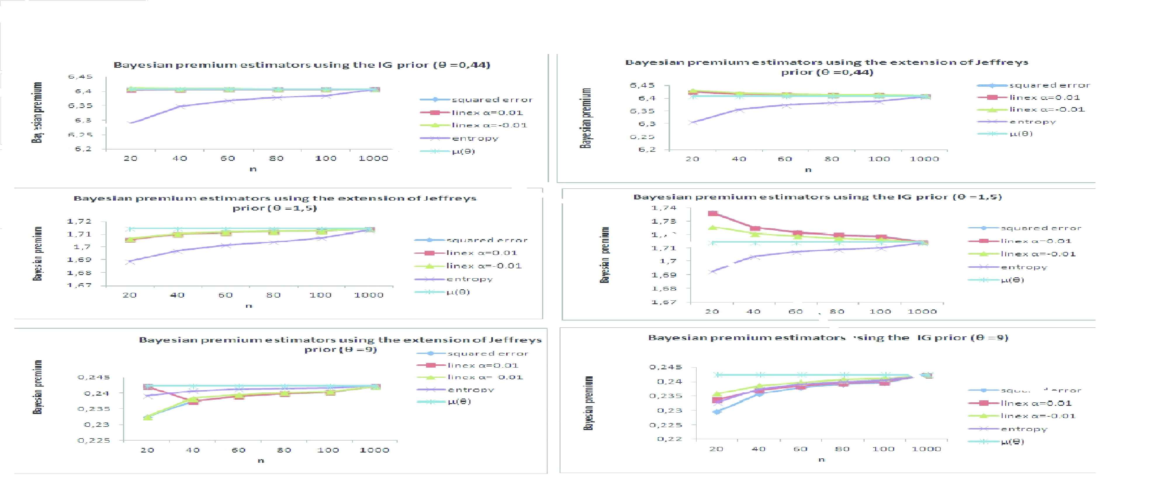
Where N is the number of replications. We generated 100,000 samples of size n =20, 40, 60, 80, 100, 1,000 and 10,000 to represent small, moderate and large sample sizes from ZD with three values of θ=0.44,1.5,9. In order to compare the Bayesian premium estimators obtained in the above section under three different loss functions and two priors, we choose the values of the extensive Jeffreys constants, (c=0.01, 0.5, 1) and for the IG prior, the following pairs of values of the hyper parameters α and β are chosen α,β=(0.2, 0.3),1,1.5 with two values of linex loss symmetry a=±0.01 and q=1 for entropy loss (Fig. 1).

The results are summarized and tabulated in the following Tables 1–4.

θ	0.44	1.5	9.0
μ(θ)	6.408346	1.714286	0.2424242
n		Ext.J.P
20	6.427768 (0.0003772195)	1.70642 (6.186881e−05)	0.2325904 (9.670397e−05)
40	6.418092 (9.499057e−05)	1.710361 (1.540085e−05)	0.2374164 (2.507806e−05)
60	6.414851 (4.232033e−05)	1.711671 (6.835437e−06)	0.239065 (1.128418e−05)
80	6.413228 (2.383403e−05)	1.712326 (3.842341e−06)	0.239897 (6.386787e−06)
100	6.412253 (1.526487e−05)	1.712718 (2.458112e−06)	0.2403987 (4.102794e−06)
1000	6.408737 (1.53049e−07)	1.714129 (2.454623e−08)	0.2422203 (4.15837e−08)
n		IG.P
20	6.408436 (8.184013e−09)	1.73643 (0.0004903582)	0.2296947 (0.0001620411)
40	6.408226 (1.427129e−08)	1.725384 (0.0001231621)	0.2359006 (4.255847e−05)
60	6.408229 (1.361046e−08)	1.72169 (5.482373e−05)	0.2380387 (1.923311e−05)
80	6.408244 (1.029034e−08)	1.719841 (3.086227e−05)	0.2391212 (1.090976e−05)
100	6.408258 (7.719616e−09)	1.718731 (1.976105e−05)	0.2397752 (7.017584e−06)
1000	6.408335 (1.256809e−10)	1.714731 (1.979417e−07)	0.2421569 (7.14696e−08)

Table 1

Bayesian premium estimators and respective MSE's under squared error loss function (α = 0.2, β = 0.3, c = 0.01)

θ	0.44	1.5	9.0
μ(θ)	6.408346	1.714286	0.2424242
n		Ext.J.P
20	6.423919 (0.0002425291)	1.706052 (6.779723e−05)	0.2325945 (9.662431e−05)
40	6.416157 (6.100882e−05)	1.710176 (1.689136e−05)	0.2374184 (2.505827e−05)
60	6.413558 (2.717113e−05)	1.711547 (7.499168e−06)	0.2390664 (1.127541e−05)
80	6.412257 (1.529957e−05)	1.712232 (4.216053e−06)	0.239898 (6.381861e−06)
100	6.411476 (9.797806e−06)	1.712643 (2.697428e−06)	0.2403995 (4.099645e−06)
1000	6.408659 (9.819732e−08)	1.714122 (2.694448e−08)	0.2422204 (4.155233e−08)
n		IG.P
20	6.404592 (1.408841e−05)	1.736061 (0.0004741641)	0.2338005 (7.436952e−05)
40	6.406292 (4.217769e−06)	1.725198 (0.000119076)	0.2371807 (2.749423e−05)
60	6.406937 (1.985068e−06)	1.721566 (5.300208e−05)	0.2386573 (1.418976e−05)
80	6.407274 (1.148483e−06)	1.719748 (2.983602e−05)	0.239485 (8.639111e−06)
100	6.407481 (7.47438e−07)	1.718656 (1.910364e−05)	0.2400145 (5.806893e−06)
1000	6.408257 (7.9315e−09)	1.714723 (1.913457e−07)	0.2421813 (5.904271e−08)

Table 2

Bayesian premium estimators and respective MSE's under linex loss function (α = 0.2, β = 0.3, a = 0.01, c = 0.5).

θ	0.44	1.5	9.0
μ(θ,γ)	6.408346	1.714286	0.2424242
n		Ext.J.P
20	6.431615 (0.0005414665)	1.706788 (5.621073e−05)	0.2325864 (9.678369e−05)
40	6.420027 (0.0001364558)	1.710547 (1.397906e−05)	0.2384016 (1.618175e−05)
60	6.416144 (6.080963e−05)	1.711795 (6.202423e−06)	0.2395387 (8.326238e−06)
80	6.414198 (3.425128e−05)	1.712419 (3.485955e−06)	0.2401746 (5.06069e−06)
100	6.41303 (2.193846e−05)	1.712792 (2.229904e−06)	0.2405809 (3.397942e−06)
1000	6.408815 (2.200214e−07)	1.714137 (2.225972e−08)	0.2422388 (3.439732e−08)
n		IG.P
20	6.41228 (1.547928e−05)	1.725569 (0.0001273162)	0.2358985 (4.258488e−05)
40	6.410161 (3.293498e−06)	1.72074 (4.165851e−05)	0.238655 (1.420682e−05)
60	6.409521 (1.382034e−06)	1.718806 (2.042952e−05)	0.2397744 (7.021747e−06)
80	6.409215 (7.548e−07)	1.7173 (9.085614e−06)	0.2406517 (3.141889e−06)
100	6.409035 (4.744779e−07)	1.716547 (5.112298e−06)	0.2410926 (1.773294e−06)
1000	6.408412 (4.440555e−09)	1.714512 (5.116727e−08)	0.2422905 (1.789591e−08)

Table 3

Bayesian premium estimators and respective MSE's under (α = 0.2, β = 0.3, a = −0.01, c = 0.5).

θ	0.44	1.5	9
μ(θ)	6.408346	1.714286	0.2424242
n		Ext.J.P
20	6.307508 (0.01016832)	1.688745 (0.0006523198)	0.2390914 (1.110798e−05)
40	6.357651 (0.002569982)	1.697218 (0.0002913227)	0.2407382 (2.842876e−06)
60	6.374487 (0.001146389)	1.701469 (0.0001642655)	0.2412957 (1.273515e−06)
80	6.382929 (0.0006460224)	1.704025 (0.0001052825)	0.2415762 (7.191958e−07)
100	6.388001 (0.0004139078)	1.707439 (4.688288e−05)	0.241745 (4.61383e−07)
1000	6.406307 (4.155459e−06)	1.713257 (1.058344e−06)	0.242356 (4.653705e−09)
n		IG.P
20	6.28851 (0.01651358)	1.693029 (0.1591305)	0.2327684 (0.01352628)
40	6.347871 (0.004780887)	1.703629 (0.1676992)	0.237462 (0.01464006)
60	6.367904 (0.002411886)	1.707175 (0.170616)	0.2390849 (0.01503543)
80	6.377967 (0.001524722)	1.70895 (0.1720858)	0.2399079 (0.01523793)
100	6.38402 (0.001088649)	1.710016 (0.1729713)	0.2404054 (0.01536101)
1000	6.405905 (0.0001234279)	1.713858 (0.1761822)	0.2422203 (0.01581417)

Table 4

Bayesian premium estimators and respective MSE's under entropy loss function (α = 1, β = 1.5, q = 1, c = 1).

DISCUSSION

This study deals with the Bayesian estimation problem based on ZD as a conditional distribution. For Bayesian premium estimators, the performance depends on the form of the prior distribution, and the loss function assumed. Most authors used squared error as a symmetric loss function. However, in practice, the real loss function is often not symmetric. The simulation study revealed that the Bayesian premium estimator under entropy loss is also more efficient than the Bayes estimator under squared error and Linex loss functions in most of the situation. Furthermore, MSE of the Bayesian premium estimators for the entropy loss has the smallest values as compared with the corresponding Bayesian estimators under Linex and squared error loss functions. It may be noted here that when θ increases, μθ decreases and the Bayesian premium estimator tends to μθ. Under the two above priors, we conclude that the performance is approximately equal to smaller posterior risk as compared. Also, the results of the gamma prior are more precise than an extension of Jeffreys prior. From the above mentioned discussion, we may conclude that the Bayes procedure discussed in this paper can be recommended for their use.

4. CONCLUSION

In this paper, since the risk parameter for a policyholder is never known, we constructed Bayesian premium estimators following Bayesian inference techniques. By imposing a prior distribution on, we are able to probabilistically describe the risk structure for the entire rating class. In practice, the choice of this prior distribution is subjective to personal judgments or induced from historical data of the corresponding group. Using numerical simulation, it seems that the Bayesian premiums are consistent and verified the condition of convergence to the individual premium. For future studies, we can consider the distributions of inverse Lindley, gamma-Lindley as a conditional distribution instead of ZD, under entropy, linex and squared error loss functions respectively. In addition, this work can be extended using censored data.

ACKNOWLEDGMENTS

The authors acknowledge Editor in chief, Prof. Mohammad Ahsanullah and the referee, of this journal for the constant encouragement to finalize the paper. Their comments and suggestions greatly improved the article.

REFERENCES

1.A.L. Bailey, Proc. Casual. Actuar. Soc., Vol. 37, 1950, pp. 7-23.

2.H. Zeghdoudi and H. Messaadia, Int. J. Comput. Sci. Math., Vol. 9, No. 1, 2018, pp. 58-65.

3.M.E. Ghitany, B. Atieh, and S. Nadarajah, Math. Comput. Simulat., Vol. 78, 2008, pp. 493-506.

4.D.V. Lindley, J. R. Stat. Soc. Ser. A., Vol. 20, 1958, pp. 102-107.

5.H. Zeghdoudi and S. Nedjar, J. Appl. Probab. Stat., Vol. 11, No. 1, 2016, pp. 129-138.

6.H. Zeghdoudi and S. Nedjar, J. Afr. Stat., Vol. 11, No. 1, 2016, pp. 923-932.

7.H. Zeghdoudi and S. Nedjar, J. Comput. Appl. Math., Vol. 298, 2016, pp. 167-174.

8.H. Zeghdoudi and S. Nedjar, J. New Trends Math. Sci., Vol. 5, No. 1, 2017, pp. 59-65.

9.H. Zeghdoudi and N. Lazri, JGSTF JMSOR., Vol. 3, No. 2, 2016, pp. 1-7.

10.R. Shanker, S. Sharma, and R. Shanker, Appl. Math., Vol. 4, No. 2, 2013, pp. 1-6.

11.A. Zellner, J. Ams. Stat. Assoc., Vol. 81, 1986, pp. 446-451.

12.M. Sankaran, Biometrics., Vol. 26, 1970, pp. 145-149.

13.M.E. Ghitany and D.K. Al-Mutairi, J. Stat. Comput. Simul., Vol. 79, No. 1, 2009, pp. 1-9.

14.H. Krishna and K. Kumar, Math. Comput. Simul., Vol. 82, No. 2, 2011, pp. 281-294.

15.S. Ali, M. Aslam, and S.M.A. Kazmi, Appl. Math. Model., Vol. 37, 2013, pp. 6068-6078.

16.F. Metiri, H. Zeghdoudi, and M.R. Remita, Global J Pure App Math., Vol. 12, No. 1, 2016, pp. 391-400.

17.A. Legendre, Nouvelles méthodes pour la determination des orbites des comètes, Courcier, City Paris, 1805.

18.H.S. Al-Kutubi and N.A. Ibrahim, Malay. J. Math. Sci., Vol. 3, No. 2, 2009, pp. 297-313.

19.D.V. Lindley, Trab. Invest. Oper., Vol. 31, No. 1, 1980, pp. 223-245.

20.H.A. Howlader and A. Hossain, Comput. Stat. Data. Anal., Vol. 38, 2002, pp. 301-314.

21.Z.F. Jaheen, J. Stat. Comput. Simul., Vol. 75, 2005, pp. 1-11.

22.Rojo, Commun. Stat. Theory Methods., Vol. 116, 1987, pp. 3745-3748.

23.A.P. Basu and N. Ebrahimi, J. Stat. Plann. Infer., Vol. 29, 1991, pp. 21-31.

24.B.N. Pandey, Commun. Stat. Theory Methods., Vol. 26, No. 9, 1997, pp. 2191-2202.

25.R.D. Thompson, A.P. Basu, and J. Bayesian, Anal. Stat. Econ., Wiley, New York, 1996.

26.M. Nassar and F.H. Eissa, Commun. Stat. Theory Methods., Vol. 33, No. 10, 2004, pp. 2343-2362.

27.R. Calabria and G. Pulcini, Commun. Stat. Theory Methods., Vol. 25, No. 3, 1969, pp. 585-600.

28.H.P. Garthwaite, B.J. Kadane, and A. O'Hagan, Elicitation, working paper in university of Sheffield, 2004.

29.S.E. Ahn, C.S. Park, and H.M. Kim, Stoch. Environ. Res. Assess., Vol. 21, 2007, pp. 711-716.

<Previous Article In Issue

Download article (PDF)

Next Article In Issue>

Journal: Journal of Statistical Theory and Applications
Volume-Issue: 17 - 4
Pages: 661 - 673
Publication Date: 2018/12/31
ISSN (Online): 2214-1766
ISSN (Print): 1538-7887
DOI: 10.2991/jsta.2018.17.4.8 How to use a DOI?
Open Access: This is an open access article under the CC BY-NC license (http://creativecommons.org/licences/by-nc/4.0/).

Cite this article

ris enw bib

TY  - JOUR
AU  - Fatma Zohra Attoui
AU  - Halim Zeghdoudi
AU  - Ahmed Saadoun
PY  - 2018
DA  - 2018/12/31
TI  - Bayesian Premium Estimators for Mixture of Two Gamma Distributions Under Squared Error, Entropy and Linex Loss Functions: With Informative and Non Informative Priors
JO  - Journal of Statistical Theory and Applications
SP  - 661
EP  - 673
VL  - 17
IS  - 4
SN  - 2214-1766
UR  - https://doi.org/10.2991/jsta.2018.17.4.8
DO  - 10.2991/jsta.2018.17.4.8
ID  - Attoui2018
ER  -

download .riscopy to clipboard