
A Comprehensive Study on Power of Tests for Normality
Corresponding author. Email: alizadehhadi@birjand.ac.ir
- DOI
- 10.2991/jsta.2018.17.4.7How to use a DOI?
- Keywords
- Test of normality; Monte Carlo simulation; Power of test; The generalized lambda distribution
- Abstract
Many statistical procedures assume that the underling distribution is normal. In this paper, we consider the popular and powerful tests for normality and investigate the power values of these tests to detect deviations from normality. The family of four-parameter generalized lambda distributions (FMKL) for its high flexibility is considered as alternative distributions. We then compare the power values of normality tests against these alternatives and for different sample sizes. The considered tests are Kolmogorov-Smirnov, Anderson-Darling, Kuiper, Jarque-Bera, Cramer von Mises, Shapiro-Wilk and Vasicek. These tests are popular tests which are commonly used in practice and statistical software. The tests are described and then power values of the tests are compared against FMKL family by Monte Carlo simulation. The results are discussed and interpreted. Finally, we apply some real data examples to show the behavior of the tests in practice.
- Copyright
- © 2018 The Authors. Published by Atlantis Press SARL.
- Open Access
- This is an open access article under the CC BY-NC license (http://creativecommons.org/licences/by-nc/4.0/).
1. INTRODUCTION
Ramberg and Schmeiser [1] introduced the four-parameter generalized lambda distribution (GLD) as
Because of the limitations of the Ramberg and Schmeiser (RS) parameterizations, Freimer et al. [2] proposed a new parameterization called FMKL as
The five different shapes of the FMKL are: unimodal, U-shaped, J-shaped, S-shaped, and monotone, which may be symmetric and asymmetric with smooth, abrupt, truncated, long, medium or short tails.
In many situations, a goodness of fit test about the distribution of the population using observations is necessary. Since the normal distribution is widely used in many statistical procedures and also is the most fundamental distribution, test for the normal hypothesis is indispensable. Moreover, testing normality is one of the most areas of statistical research. For example in statistical modeling the normal assumption of the underlying error distribution must be checked. Therefore, many tests for normality are proposed by authors. A fair of normality tests can be found in the statistical literature. In many situations, a goodness of fit test about the distribution of the population is necessary. Since the normal distribution is the most basic distribution and use widely in statistics, test for the normal hypothesis has been studied by many authors. See for example, D'Agostino and Stephens [3], Huber-Carol et al. [4], Thode [5].
Recently, testing normality has been considered by Alizadeh Noughabi and Arghami [6], Harri and Coble [7], Sanqui et al. [8], Zamanzade and Arghami [9], Marmolejo-Ramos and González-Burgos [10], Joenssen and Vogel [11] and Wang [12].
In this article, we consider seven popular (like Kolmogorov-Smirnov, Anderson-Darling) and powerfulness (like Shapiro-Wilk, Vasicek) normality tests and compare power values of these tests against the GLD (FMKL) with different parameters. We show that no single test procedure is uniformly more powerful than others. However, the powerful tests can be determined based on type of alternatives. Thus, tests for normality based on type of alternatives are classified.
The methodologies of the considered tests are presented in Section 2. Power values of the tests are compared with each other against the FMKL family by Monte Carlo simulation in Section 3. In Section 4, the applicability of the tests in practice is shown by real data. Finally, some conclusions are given in Section 5.
2. TESTS FOR NORMALITY
Given a random sample
In this section, we consider seven popular tests for the above hypothesis. The considered tests are Cramer von Mises [13], Kolmogorov-Smirnov [14], Anderson-Darling [15], Kuiper [16], Shapiro-Wilk [17], Vasicek [18] and Jarque-Bera [19]. These tests are commonly used in practice and software. For example, the Shapiro-Wilks test is used in SAS software for testing normality. The description of each normality tests is presented in Table 1.
| Test of normality | Test statistic | Notations |
|---|---|---|
| 1- Cramer von Mises | ||
| 2- Kolmogorov-Smirnov | ||
| 3- Kuiper | D+ and D− are as above. | |
| 4- Shapiro-Wilk | The coefficients ai are tabulated in Pearson and Hartley [20] | |
| 5- Anderson-Darling | ||
| 6- Vasicek | ||
| 7- Jarque-Bera |
Tests of normality.
From the aforementioned tests, Vasicek's test, Shapiro-Wilk and Jarque-Bera test are specific in the sense that the null hypothesis is normal, while the rest are suitable for any null family of distributions. For further study about this tests, see D'Agostino and Stephens [3] and references there in.
3. SIMULATION STUDY
In this section, Type I error of the tests are obtained and then power values of the tests against flexible FMKL family are computed through a Monte Carlo simulation.
3.1 Type I Error of the Tests
Through a Monte Carlo simulation, we compute Type I error of the tests. Table 2 presents Type I error probabilities (the actual size of the tests), which have been obtained by 20,000 simulations. As is evident from Table 2 the actual size of the tests are quite acceptable.
| Test of normality | σ = .01 | σ = .25 | σ = 1 | σ = 5 | σ = 10 | σ = 100 |
|---|---|---|---|---|---|---|
| Cramer von Mises | 0.0510 | 0.0506 | 0.0498 | 0.0492 | 0.0485 | 0.0509 |
| Kolmogorov-Smirnov | 0.0507 | 0.0492 | 0.0503 | 0.0505 | 0.0491 | 0.0511 |
| Kuiper | 0.0517 | 0.0509 | 0.0501 | 0.0493 | 0.0508 | 0.0487 |
| Shapiro-Wilk | 0.0503 | 0.0497 | 0.0499 | 0.0504 | 0.0497 | 0.0501 |
| Anderson-Darling | 0.0491 | 0.0505 | 0.0497 | 0.0506 | 0.0490 | 0.0508 |
| Vasicek | 0.0498 | 0.0501 | 0.0503 | 0.0499 | 0.0502 | 0.0496 |
| Jarque-Bera | 0.0503 | 0.0495 | 0.0501 | 0.0499 | 0.0502 | 0.0501 |
Actual sizes of the tests for nominal significance level α = 0.05 (n = 20, σ = standard deviation).
3.2 Shapes of FMKL Family
The shapes returned by FMKL family are classified by Freimer et al. [2] as follows.
Class I
Class Ia
Class Ib
Class Ic
Class II
Class III
Class IV
Class V
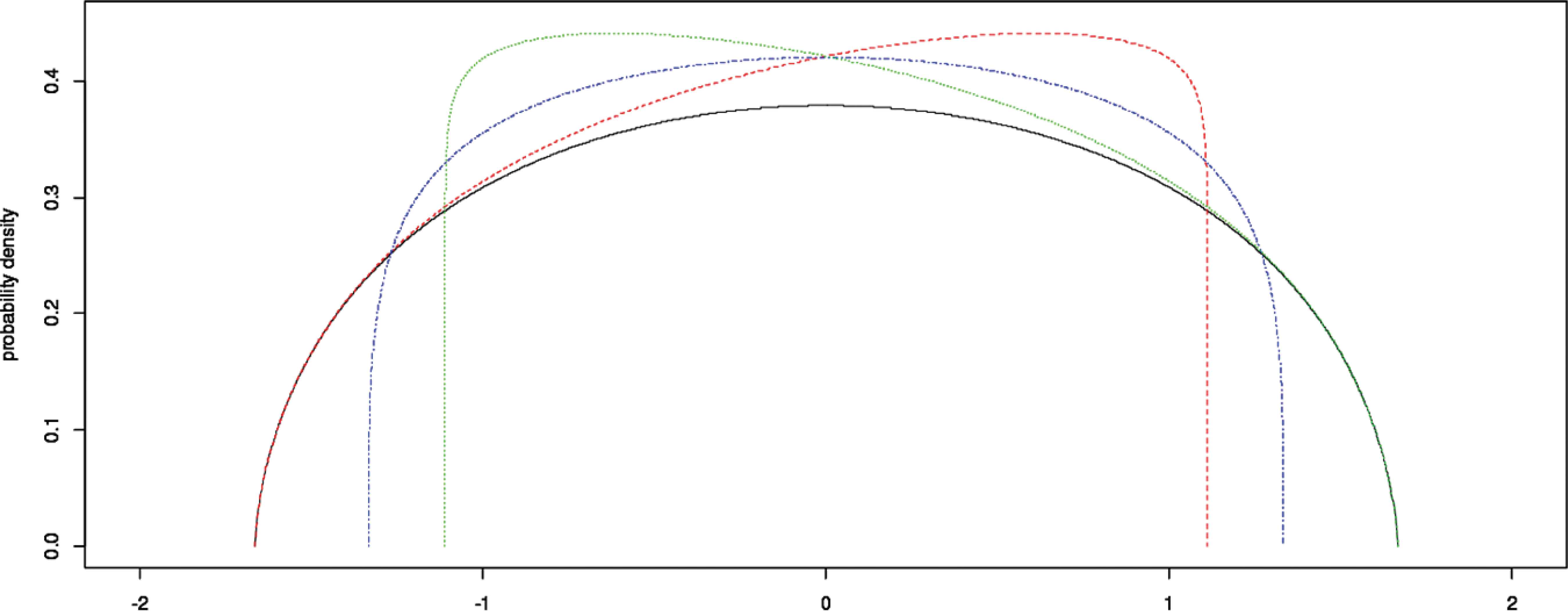
Examples of each class of shapes are displayed in Figs. 1–7.
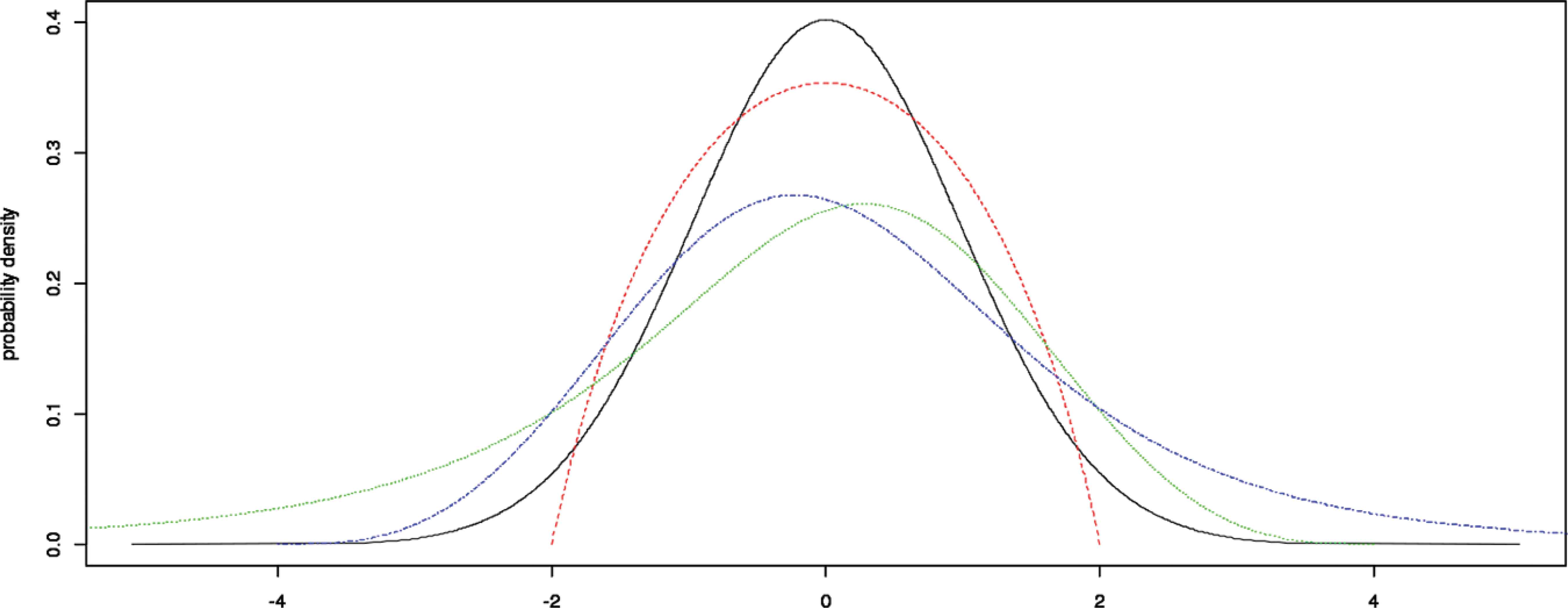
Class Ia pdfs including the normal distribution.

Class Ib pdfs.
Class Ic pdfs.

Class II pdfs includes the exponential distribution.
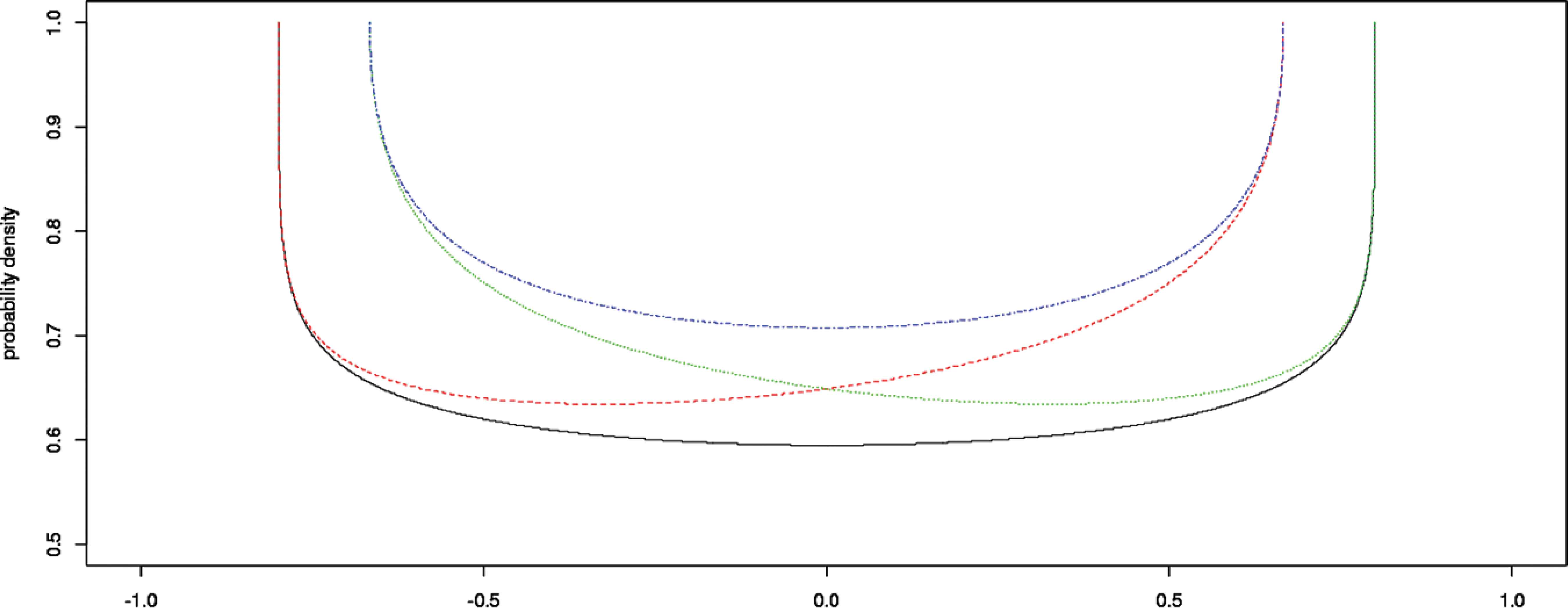
Class III U-shaped pdfs.
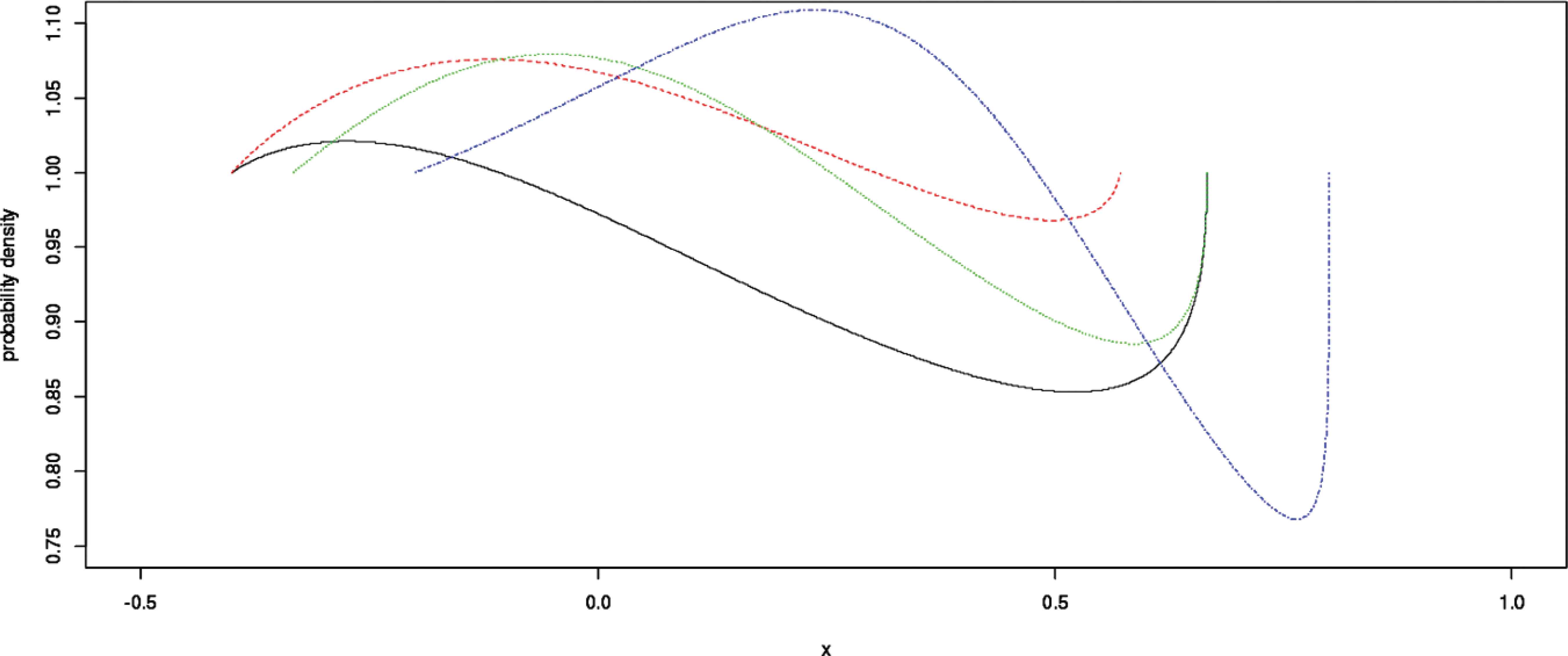
Class IV S-shaped pdfs.

Class V pdfs.
3.3 Power Comparison
To comparison of the power values of the tests, we select alternatives from FMKL family with different parameters. We compute the power values of the tests based on CH, D, V, W, A2, KLmn and JB statistics against FMKL family by means of Monte Carlo simulations. As mentioned above, the alternatives can divide into five groups (Class I to V).
Power values of the tests were obtained by simulation in the following manner.
Under each alternative we generated 20,000 samples of size 10, 20, 30, 50. We calculated for each sample the statistics (CH, D, V, W, A2, KLmn, JB) and the power value of the corresponding test was computed by the frequency of the event “the value of the test statistic is in the critical region”. The required critical regions are given in the corresponding articles, but we obtained them by simulation, before power simulations. The power values of the tests are presented in Tables 3–9. For each sample size and alternative, the bold type in these Tables indicates the test achieving the maximal power. For Vasicek's test, we used the recommended window sizes proposed by Vasicek [18], i.e., m = 2, (3), 4 for sample sizes n = 10, (20, 30), 50, respectively.
| n | λ3 | λ4 | α3 | α4 | D | V | CH | A2 | KLmn | W | JB |
|---|---|---|---|---|---|---|---|---|---|---|---|
| 10 | −0.2 | −0.2 | 0 | 22.21 | 0.1528 | 0.1549 | 0.1735 | 0.1780 | 0.0866 | 0.1771 | 0.2036 |
| 0.25 | 0.25 | 0 | 2.54 | 0.0457 | 0.0463 | 0.0461 | 0.0441 | 0.0558 | 0.0427 | 0.0331 | |
| 0.5 | 0.5 | 0 | 2.08 | 0.0464 | 0.0479 | 0.0452 | 0.0459 | 0.0876 | 0.0454 | 0.0227 | |
| −0.2 | −0.1 | 2.63 | 35.40 | 0.1313 | 0.1315 | 0.1467 | 0.1512 | 0.0787 | 0.1507 | 0.1736 | |
| −0.2 | 0 | 4.65 | 73.8 | 0.1278 | 0.1280 | 0.1419 | 0.1474 | 0.0843 | 0.1519 | 0.1743 | |
| −0.2 | 0.25 | 6.99 | 157.98 | 0.1546 | 0.1561 | 0.1792 | 0.1879 | 0.1309 | 0.1994 | 0.2097 | |
| −0.2 | 0.5 | 7.25 | 189.98 | 0.2075 | 0.2184 | 0.2480 | 0.2616 | 0.2083 | 0.2811 | 0.2780 | |
| 0 | −0.1 | −2.81 | 17.83 | 0.0931 | 0.0938 | 0.1017 | 0.1057 | 0.0653 | 0.1097 | 0.1277 | |
| 0 | 0.25 | 1.05 | 3.70 | 0.0765 | 0.0741 | 0.0830 | 0.0872 | 0.664 | 0.0907 | 0.0944 | |
| 0 | 0.5 | 0.566 | 2.40 | 0.1063 | 0.1092 | 0.1263 | 0.1340 | 0.1116 | 0.1438 | 0.1425 | |
| 0.25 | −0.1 | −2.13 | 11.21 | 0.1071 | 0.1043 | 0.1226 | 0.1292 | 0.0888 | 0.1360 | 0.1478 | |
| 0.25 | 0.5 | −0.041 | 2.25 | 0.0509 | 0.0538 | 0.0540 | 0.0530 | 0.0769 | 0.0533 | 0.0363 | |
| 0.5 | −0.1 | −1.15 | 4.09 | 0.1513 | 0.1562 | 0.1777 | 0.1908 | 0.1486 | 0.2052 | 0.2050 | |
| 20 | −0.2 | −0.2 | 0 | 22.21 | 0.2405 | 0.2575 | 0.2906 | 0.3083 | 0.1376 | 0.3224 | 0.3672 |
| 0.25 | 0.25 | 0 | 2.54 | 0.0464 | 0.0488 | 0.0447 | 0.0419 | 0.0668 | 0.0377 | 0.0186 | |
| 0.5 | 0.5 | 0 | 2.08 | 0.0501 | 0.0692 | 0.0612 | 0.0657 | 0.1628 | 0.0649 | 0.0064 | |
| −0.2 | −0.1 | 2.63 | 35.40 | 0.1955 | 0.2089 | 0.2391 | 0.2543 | 0.1131 | 0.2657 | 0.3110 | |
| −0.2 | 0 | 4.65 | 73.8 | 0.1914 | 0.1970 | 0.2303 | 0.2485 | 0.1281 | 0.2684 | 0.3047 | |
| −0.2 | 0.25 | 6.99 | 157.98 | 0.2755 | 0.2729 | 0.3330 | 0.3613 | 0.2637 | 0.4003 | 0.4123 | |
| −0.2 | 0.5 | 7.25 | 189.98 | 0.3790 | 0.4069 | 0.4731 | 0.5137 | 0.4726 | 0.5747 | 0.5334 | |
| 0 | −0.1 | −2.81 | 17.83 | 0.1195 | 0.1257 | 0.1436 | 0.1566 | 0.0712 | 0.1747 | 0.2127 | |
| 0 | 0.25 | 1.05 | 3.70 | 0.0981 | 0.0925 | 0.1119 | 0.1231 | 0.0908 | 0.1481 | 0.1627 | |
| 0 | 0.5 | 0.566 | 2.40 | 0.1741 | 0.1744 | 0.2234 | 0.2496 | 0.2360 | 0.3039 | 0.2719 | |
| 0.25 | −0.1 | −2.13 | 11.21 | 0.1738 | 0.1688 | 0.2091 | 0.2309 | 0.1564 | 0.2661 | 0.2822 | |
| 0.25 | 0.5 | −0.041 | 2.25 | 0.0664 | 0.0686 | 0.0738 | 0.0773 | 0.1322 | 0.0807 | 0.0375 | |
| 0.5 | −0.1 | −1.15 | 4.09 | 0.2680 | 0.2819 | 0.3443 | 0.3824 | 0.3481 | 0.4431 | 0.4049 | |
| 30 | −0.2 | −0.2 | 0 | 22.21 | 0.3199 | 0.3535 | 0.3903 | 0.4132 | 0.2093 | 0.4289 | 0.4805 |
| 0.25 | 0.25 | 0 | 2.54 | 0.0449 | 0.0502 | 0.0480 | 0.0444 | 0.0741 | 0.0365 | 0.0105 | |
| 0.5 | 0.5 | 0 | 2.08 | 0.0653 | 0.0937 | 0.0849 | 0.0934 | 0.2309 | 0.0986 | 0.0028 | |
| −0.2 | −0.1 | 2.63 | 35.40 | 0.2695 | 0.2970 | 0.3300 | 0.3527 | 0.1789 | 0.3711 | 0.4263 | |
| −0.2 | 0 | 4.65 | 73.8 | 0.2668 | 0.2774 | 0.3254 | 0.3470 | 0.1962 | 0.3763 | 0.4219 | |
| −0.2 | 0.25 | 6.99 | 157.98 | 0.3847 | 0.3763 | 0.4599 | 0.4975 | 0.3857 | 0.5528 | 0.5561 | |
| −0.2 | 0.5 | 7.25 | 189.98 | 0.5343 | 0.5667 | 0.6508 | 0.6999 | 0.6765 | 0.7739 | 0.7052 | |
| 0 | −0.1 | −2.81 | 17.83 | 0.1556 | 0.1656 | 0.1919 | 0.2087 | 0.1006 | 0.2288 | 0.2744 | |
| 0 | 0.25 | 1.05 | 3.70 | 0.1292 | 0.1153 | 0.1526 | 0.1687 | 0.1196 | 0.2096 | 0.2200 | |
| 0 | 0.5 | 0.566 | 2.40 | 0.2589 | 0.2591 | 0.3383 | 0.3878 | 0.3729 | 0.4775 | 0.3946 | |
| 0.25 | −0.1 | −2.13 | 11.21 | 0.2399 | 0.2235 | 0.2933 | 0.3236 | 0.2312 | 0.3816 | 0.3894 | |
| 0.25 | 0.5 | −0.041 | 2.25 | 0.0867 | 0.0862 | 0.0996 | 0.1076 | 0.1776 | 0.1133 | 0.0354 | |
| 0.5 | −0.1 | −1.15 | 4.09 | 0.3914 | 0.4127 | 0.5011 | 0.5576 | 0.5337 | 0.6466 | 0.5699 | |
| 50 | −0.2 | −0.2 | 0 | 22.21 | 0.4480 | 0.5077 | 0.5451 | 0.5780 | 0.3270 | 0.6084 | 0.6562 |
| 0.25 | 0.25 | 0 | 2.54 | 0.0497 | 0.0552 | 0.0527 | 0.0523 | 0.0918 | 0.0437 | 0.0068 | |
| 0.5 | 0.5 | 0 | 2.08 | 0.0966 | 0.1521 | 0.1396 | 0.1691 | 0.4101 | 0.2094 | 0.0095 | |
| −0.2 | −0.1 | 2.63 | 35.40 | 0.3738 | 0.4194 | 0.4624 | 0.4946 | 0.2648 | 0.5398 | 0.5927 | |
| −0.2 | 0 | 4.65 | 73.8 | 0.3797 | 0.3957 | 0.4563 | 0.4879 | 0.2910 | 0.5347 | 0.5831 | |
| −0.2 | 0.25 | 6.99 | 157.98 | 0.5622 | 0.5449 | 0.6537 | 0.7002 | 0.5894 | 0.7737 | 0.7631 | |
| −0.2 | 0.5 | 7.25 | 189.98 | 0.7513 | 0.7961 | 0.8586 | 0.9030 | 0.9016 | 0.9484 | 0.9003 | |
| 0 | −0.1 | −2.81 | 17.83 | 0.2081 | 0.2310 | 0.2669 | 0.2969 | 0.1355 | 0.3465 | 0.4017 | |
| 0 | 0.25 | 1.05 | 3.70 | 0.1811 | 0.1511 | 0.2195 | 0.2494 | 0.1819 | 0.3327 | 0.3312 | |
| 0 | 0.5 | 0.566 | 2.40 | 0.3920 | 0.3995 | 0.5127 | 0.5946 | 0.6172 | 0.7340 | 0.5962 | |
| 0.25 | −0.1 | −2.13 | 11.21 | 0.3529 | 0.3282 | 0.4396 | 0.4870 | 0.3692 | 0.5861 | 0.5811 | |
| 0.25 | 0.5 | −0.041 | 2.25 | 0.1242 | 0.1237 | 0.1525 | 0.1777 | 0.2961 | 0.2181 | 0.0505 | |
| 0.5 | −0.1 | −1.15 | 4.09 | 0.5807 | 0.6176 | 0.7171 | 0.7848 | 0.7895 | 0.8772 | 0.7932 |
Power comparisons of the tests at significance level 0.05 for sample sizes n = 10, 20, 30 and 50 under alternatives from group Ia.
| n | λ3 | λ4 | α3 | α4 | D | V | CH | A2 | KLmn | W | JB |
|---|---|---|---|---|---|---|---|---|---|---|---|
| 10 | 0.6 | −0.2 | −7.26 | 198.82 | 0.2239 | 0.2423 | 0.2734 | 0.2894 | 0.2451 | 0.3098 | 0.2951 |
| 0.6 | −0.1 | −0.94 | 3.29 | 0.1687 | 0.1799 | 0.2047 | 0.2190 | 0.1846 | 0.2398 | 0.2266 | |
| 0.6 | 0 | −0.42 | 2.16 | 0.1222 | 0.1292 | 0.1457 | 0.1556 | 0.1400 | 0.1704 | 0.1624 | |
| 0.6 | 0.25 | 0.094 | 2.18 | 0.0595 | 0.0607 | 0.0639 | 0.0662 | 0.0942 | 0.0691 | 0.0492 | |
| 0.6 | 0.5 | 0.045 | 2.03 | 0.0446 | 0.0515 | 0.0469 | 0.0486 | 0.0941 | 0.0479 | 0.0221 | |
| 0.75 | −0.2 | −7.33 | 212.90 | 0.2540 | 0.2866 | 0.3140 | 0.3339 | 0.3070 | 0.3631 | 0.3360 | |
| 0.75 | −0.1 | −0.69 | 2.60 | 0.1926 | 0.2121 | 0.2406 | 0.2584 | 0.2373 | 0.2809 | 0.2614 | |
| 0.75 | 0 | −0.24 | 1.95 | 0.1447 | 0.1587 | 0.1805 | 0.1925 | 0.1837 | 0.2120 | 0.1953 | |
| 0.75 | 0.25 | 0.18 | 2.12 | 0.0757 | 0.0801 | 0.0833 | 0.0871 | 0.1201 | 0.0929 | 0.0681 | |
| 0.75 | 0.5 | 0.12 | 1.99 | 0.0534 | 0.0605 | 0.0563 | 0.0583 | 0.1109 | 0.0579 | 0.0294 | |
| 0.9 | −0.2 | −7.49 | 229.48 | 0.2764 | 0.3180 | 0.3471 | 0.3689 | 0.3569 | 0.4001 | 0.3577 | |
| 0.9 | −0.1 | −0.49 | 2.20 | 0.2223 | 0.2554 | 0.2803 | 0.2993 | 0.2882 | 0.3257 | 0.2921 | |
| 0.9 | 0 | −0.09 | 1.84 | 0.1673 | 0.1906 | 0.2109 | 0.2278 | 0.2290 | 0.2482 | 0.2186 | |
| 0.9 | 0.25 | 0.26 | 2.11 | 0.0913 | 0.0995 | 0.1047 | 0.1121 | 0.1460 | 0.1220 | 0.0869 | |
| 0.9 | 0.5 | 0.19 | 1.97 | 0.0633 | 0.0747 | 0.0710 | 0.0739 | 0.1349 | 0.0780 | 0.0397 | |
| 20 | 0.6 | −0.2 | −7.26 | 198.82 | 0.4219 | 0.4648 | 0.5269 | 0.5732 | 0.5592 | 0.6399 | 0.5715 |
| 0.6 | −0.1 | −0.94 | 3.29 | 0.3120 | 0.3412 | 0.4032 | 0.4495 | 0.4458 | 0.5179 | 0.4501 | |
| 0.6 | 0 | −0.42 | 2.16 | 0.2105 | 0.2228 | 0.2727 | 0.3105 | 0.3202 | 0.3750 | 0.3107 | |
| 0.6 | 0.25 | 0.094 | 2.18 | 0.0843 | 0.0886 | 0.0988 | 0.1083 | 0.1745 | 0.1209 | 0.0550 | |
| 0.6 | 0.5 | 0.045 | 2.03 | 0.0582 | 0.0787 | 0.0710 | 0.0755 | 0.1849 | 0.0763 | 0.0061 | |
| 0.75 | −0.2 | −7.33 | 212.90 | 0.4789 | 0.5543 | 0.6034 | 0.6534 | 0.6786 | 0.7196 | 0.6282 | |
| 0.75 | −0.1 | −0.69 | 2.60 | 0.3719 | 0.4323 | 0.4801 | 0.5309 | 0.5751 | 0.6107 | 0.5143 | |
| 0.75 | 0 | −0.24 | 1.95 | 0.2621 | 0.3037 | 0.3553 | 0.4024 | 0.4517 | 0.4827 | 0.3776 | |
| 0.75 | 0.25 | 0.18 | 2.12 | 0.1165 | 0.1257 | 0.1473 | 0.1640 | 0.2680 | 0.1927 | 0.0905 | |
| 0.75 | 0.5 | 0.12 | 1.99 | 0.0759 | 0.1001 | 0.0943 | 0.1053 | 0.2443 | 0.1145 | 0.0126 | |
| 0.9 | −0.2 | −7.49 | 229.48 | 0.5260 | 0.6127 | 0.6513 | 0.6996 | 0.7457 | 0.7658 | 0.6586 | |
| 0.9 | −0.1 | −0.49 | 2.20 | 0.4261 | 0.5124 | 0.5553 | 0.6099 | 0.6801 | 0.6868 | 0.5609 | |
| 0.9 | 0 | −0.09 | 1.84 | 0.3172 | 0.3835 | 0.4262 | 0.4784 | 0.5613 | 0.5623 | 0.4276 | |
| 0.9 | 0.25 | 0.26 | 2.11 | 0.1477 | 0.1674 | 0.1954 | 0.2236 | 0.3580 | 0.2680 | 0.1264 | |
| 0.9 | 0.5 | 0.19 | 1.97 | 0.0949 | 0.1212 | 0.1220 | 0.1406 | 0.3147 | 0.1610 | 0.0245 | |
| 30 | 0.6 | −0.2 | −7.26 | 198.82 | 0.5934 | 0.6519 | 0.7169 | 0.7668 | 0.7718 | 0.8354 | 0.7499 |
| 0.6 | −0.1 | −0.94 | 3.29 | 0.4511 | 0.4982 | 0.5795 | 0.6416 | 0.6520 | 0.7308 | 0.6246 | |
| 0.6 | 0 | −0.42 | 2.16 | 0.3098 | 0.3333 | 0.4146 | 0.4781 | 0.5053 | 0.5834 | 0.4624 | |
| 0.6 | 0.25 | 0.094 | 2.18 | 0.1205 | 0.1212 | 0.1474 | 0.1652 | 0.2653 | 0.1912 | 0.0620 | |
| 0.6 | 0.5 | 0.045 | 2.03 | 0.0805 | 0.1122 | 0.1061 | 0.1189 | 0.2861 | 0.1281 | 0.0043 | |
| 0.75 | −0.2 | −7.33 | 212.90 | 0.6659 | 0.7511 | 0.7929 | 0.8412 | 0.8734 | 0.8981 | 0.8023 | |
| 0.75 | −0.1 | −0.69 | 2.60 | 0.5417 | 0.6214 | 0.6830 | 0.7461 | 0.7896 | 0.8241 | 0.6938 | |
| 0.75 | 0 | −0.24 | 1.95 | 0.4024 | 0.4666 | 0.5349 | 0.6067 | 0.6774 | 0.7111 | 0.5350 | |
| 0.75 | 0.25 | 0.18 | 2.12 | 0.1742 | 0.1840 | 0.2267 | 0.2652 | 0.4118 | 0.3261 | 0.1180 | |
| 0.75 | 0.5 | 0.12 | 1.99 | 0.1069 | 0.1420 | 0.1491 | 0.1752 | 0.3886 | 0.2025 | 0.0116 | |
| 0.9 | −0.2 | −7.49 | 229.48 | 0.7231 | 0.8172 | 0.8443 | 0.8878 | 0.9296 | 0.9356 | 0.8355 | |
| 0.9 | −0.1 | −0.49 | 2.20 | 0.6087 | 0.7052 | 0.7479 | 0.8078 | 0.8695 | 0.8784 | 0.7382 | |
| 0.9 | 0 | −0.09 | 1.84 | 0.4727 | 0.5774 | 0.6254 | 0.6976 | 0.7937 | 0.7981 | 0.6065 | |
| 0.9 | 0.25 | 0.26 | 2.11 | 0.2332 | 0.2681 | 0.3154 | 0.3724 | 0.5553 | 0.4579 | 0.1776 | |
| 0.9 | 0.5 | 0.19 | 1.97 | 0.1454 | 0.1909 | 0.2056 | 0.2475 | 0.4999 | 0.2963 | 0.0253 | |
| 50 | 0.6 | −0.2 | −7.26 | 198.82 | 0.8089 | 0.8683 | 0.9064 | 0.9419 | 0.9561 | 0.9758 | 0.9312 |
| 0.6 | −0.1 | −0.94 | 3.29 | 0.6671 | 0.7373 | 0.8026 | 0.8672 | 0.8979 | 0.9378 | 0.8517 | |
| 0.6 | 0 | −0.42 | 2.16 | 0.4852 | 0.5344 | 0.6301 | 0.7168 | 0.7781 | 0.8425 | 0.6888 | |
| 0.6 | 0.25 | 0.094 | 2.18 | 0.1834 | 0.1859 | 0.2449 | 0.2908 | 0.4652 | 0.3788 | 0.1042 | |
| 0.6 | 0.5 | 0.045 | 2.03 | 0.1144 | 0.1770 | 0.1741 | 0.2184 | 0.5080 | 0.2845 | 0.0188 | |
| 0.75 | −0.2 | −7.33 | 212.90 | 0.8758 | 0.9351 | 0.9514 | 0.9734 | 0.9880 | 0.9916 | 0.9596 | |
| 0.75 | −0.1 | −0.69 | 2.60 | 0.7653 | 0.8572 | 0.8882 | 0.9345 | 0.9669 | 0.9772 | 0.9053 | |
| 0.75 | 0 | −0.24 | 1.95 | 0.6089 | 0.7146 | 0.7725 | 0.8515 | 0.9194 | 0.9356 | 0.7887 | |
| 0.75 | 0.25 | 0.18 | 2.12 | 0.2825 | 0.3179 | 0.3852 | 0.4729 | 0.6954 | 0.6126 | 0.2144 | |
| 0.75 | 0.5 | 0.12 | 1.99 | 0.1714 | 0.2372 | 0.2559 | 0.3257 | 0.6598 | 0.4337 | 0.0422 | |
| 0.9 | −0.2 | −7.49 | 229.48 | 0.9219 | 0.9685 | 0.9734 | 0.9884 | 0.9964 | 0.9974 | 0.9756 | |
| 0.9 | −0.1 | −0.49 | 2.20 | 0.8404 | 0.9238 | 0.9354 | 0.9674 | 0.9895 | 0.9907 | 0.9390 | |
| 0.9 | 0 | −0.09 | 1.84 | 0.7120 | 0.8372 | 0.8610 | 0.9229 | 0.9743 | 0.9767 | 0.8601 | |
| 0.9 | 0.25 | 0.26 | 2.11 | 0.3854 | 0.4586 | 0.5274 | 0.6340 | 0.8434 | 0.7846 | 0.3480 | |
| 0.9 | 0.5 | 0.19 | 1.97 | 0.2419 | 0.3130 | 0.3565 | 0.4512 | 0.7868 | 0.5925 | 0.0852 |
Power comparisons of the tests at significance level 0.05 for sample sizes n = 10, 20, 30 and 50 under alternatives from group Ib.
| n | λ3 | λ4 | α3 | α4 | D | V | CH | A2 | KLmn | W | JB |
|---|---|---|---|---|---|---|---|---|---|---|---|
| 10 | 0.6 | 0.6 | 0 | 1.99 | 0.0494 | 0.0587 | 0.0519 | 0.0525 | 0.1019 | 0.0508 | 0.0230 |
| 0.6 | 0.9 | −0.14 | 1.92 | 0.0608 | 0.0715 | 0.0678 | 0.0704 | 0.1384 | 0.0744 | 0.0321 | |
| 0.75 | 0.6 | 0.07 | 1.94 | 0.0514 | 0.0612 | 0.0563 | 0.0583 | 0.1167 | 0.0590 | 0.0258 | |
| 0.75 | 0.75 | 0 | 1.89 | 0.0550 | 0.0690 | 0.0621 | 0.0638 | 0.1283 | 0.0640 | 0.0250 | |
| 0.75 | 0.9 | −0.07 | 1.86 | 0.0586 | 0.0736 | 0.0661 | 0.0678 | 0.1414 | 0.0693 | 0.0261 | |
| 0.9 | 0.9 | 0 | 1.83 | 0.0594 | 0.0769 | 0.0683 | 0.0709 | 0.1518 | 0.0737 | 0.0269 | |
| 20 | 0.6 | 0.6 | 0 | 1.99 | 0.0614 | 0.0866 | 0.0791 | 0.0871 | 0.2162 | 0.0866 | 0.0053 |
| 0.6 | 0.9 | −0.14 | 1.92 | 0.0908 | 0.1216 | 0.1187 | 0.1349 | 0.3255 | 0.1536 | 0.0123 | |
| 0.75 | 0.6 | 0.07 | 1.94 | 0.0707 | 0.0994 | 0.0931 | 0.1029 | 0.2637 | 0.1110 | 0.0070 | |
| 0.75 | 0.75 | 0 | 1.89 | 0.0739 | 0.1115 | 0.1018 | 0.1167 | 0.3050 | 0.1303 | 0.0066 | |
| 0.75 | 0.9 | −0.07 | 1.86 | 0.0852 | 0.1247 | 0.1184 | 0.1387 | 0.3531 | 0.1583 | 0.0088 | |
| 0.9 | 0.9 | 0 | 1.83 | 0.0889 | 0.1339 | 0.1255 | 0.1495 | 0.3830 | 0.1743 | 0.0066 | |
| 30 | 0.6 | 0.6 | 0 | 1.99 | 0.0819 | 0.1255 | 0.1143 | 0.1353 | 0.3322 | 0.1498 | 0.0031 |
| 0.6 | 0.9 | −0.14 | 1.92 | 0.1267 | 0.1803 | 0.1876 | 0.2284 | 0.5056 | 0.2760 | 0.0124 | |
| 0.75 | 0.6 | 0.07 | 1.94 | 0.1010 | 0.1483 | 0.1440 | 0.1755 | 0.4253 | 0.2066 | 0.0063 | |
| 0.75 | 0.75 | 0 | 1.89 | 0.1079 | 0.1763 | 0.1654 | 0.2035 | 0.4877 | 0.2465 | 0.0058 | |
| 0.75 | 0.9 | −0.07 | 1.86 | 0.1266 | 0.1955 | 0.1931 | 0.2407 | 0.5529 | 0.2966 | 0.0094 | |
| 0.9 | 0.9 | 0 | 1.83 | 0.1304 | 0.2121 | 0.2101 | 0.2660 | 0.6005 | 0.3292 | 0.0105 | |
| 50 | 0.6 | 0.6 | 0 | 1.99 | 0.1228 | 0.2037 | 0.1969 | 0.2546 | 0.5836 | 0.3422 | 0.0204 |
| 0.6 | 0.9 | −0.14 | 1.92 | 0.2169 | 0.3165 | 0.3411 | 0.4448 | 0.8110 | 0.5892 | 0.0777 | |
| 0.75 | 0.6 | 0.07 | 1.94 | 0.1653 | 0.2574 | 0.2627 | 0.3424 | 0.7086 | 0.4626 | 0.0455 | |
| 0.75 | 0.75 | 0 | 1.89 | 0.1770 | 0.2964 | 0.3009 | 0.3944 | 0.7868 | 0.5399 | 0.0577 | |
| 0.75 | 0.9 | −0.07 | 1.86 | 0.2163 | 0.3457 | 0.3596 | 0.4695 | 0.8470 | 0.6249 | 0.0908 | |
| 0.9 | 0.9 | 0 | 1.83 | 0.2273 | 0.3696 | 0.3847 | 0.5076 | 0.8852 | 0.6821 | 0.1092 |
Power comparisons of the tests at significance level 0.05 for sample sizes n = 10, 20, 30 and 50 under alternatives from group Ic.
| n | λ3 | λ4 | α3 | α4 | D | V | CH | A2 | KLmn | W | JB |
|---|---|---|---|---|---|---|---|---|---|---|---|
| 10 | 1.25 | −0.2 | −8.16 | 280.37 | 0.3265 | 0.3885 | 0.4109 | 0.4369 | 0.4507 | 0.4708 | 0.4064 |
| 1.25 | −0.1 | −0.14 | 1.81 | 0.2700 | 0.3236 | 0.3481 | 0.3722 | 0.3875 | 0.4037 | 0.3448 | |
| 1.25 | 0 | 0.20 | 1.80 | 0.2153 | 0.2567 | 0.2775 | 0.2998 | 0.3207 | 0.3293 | 0.2718 | |
| 1.25 | 0.25 | 0.44 | 2.17 | 0.1251 | 0.1417 | 0.1524 | 0.1630 | 0.2148 | 0.1792 | 0.1259 | |
| 1.25 | 0.5 | 0.35 | 2.00 | 0.0841 | 0.1006 | 0.1002 | 0.1080 | 0.1861 | 0.1159 | 0.0609 | |
| 1.25 | 0.75 | 0.218 | 1.86 | 0.0715 | 0.0907 | 0.0852 | 0.0892 | 0.1768 | 0.0944 | 0.0394 | |
| 1.25 | 0.95 | 0.12 | 1.80 | 0.0658 | 0.0849 | 0.0793 | 0.0846 | 0.1808 | 0.0934 | 0.0348 | |
| 2 | −0.2 | −10.64 | 443.42 | 0.3924 | 0.4727 | 0.4942 | 0.5218 | 0.5579 | 0.5563 | 0.4749 | |
| 2 | −0.1 | 0.376 | 1.85 | 0.3283 | 0.3984 | 0.4228 | 0.4486 | 0.4854 | 0.4824 | 0.4028 | |
| 2 | 0 | 0.64 | 2.14 | 0.2761 | 0.3349 | 0.3562 | 0.3815 | 0.4211 | 0.4168 | 0.3395 | |
| 2 | 0.25 | 0.75 | 2.5 | 0.1712 | 0.2042 | 0.2191 | 0.2372 | 0.2952 | 0.2598 | 0.1867 | |
| 2 | 0.5 | 0.61 | 2.24 | 0.1190 | 0.1389 | 0.1423 | 0.1535 | 0.2292 | 0.1651 | 0.0948 | |
| 2 | 0.75 | 0.46 | 2.02 | 0.0879 | 0.1096 | 0.1082 | 0.1153 | 0.2067 | 0.1249 | 0.0559 | |
| 2 | 0.95 | 0.36 | 1.91 | 0.0773 | 0.0965 | 0.0923 | 0.1000 | 0.1968 | 0.1075 | 0.0445 | |
| 20 | 1.25 | −0.2 | −8.16 | 280.37 | 0.6143 | 0.7226 | 0.7500 | 0.7978 | 0.8623 | 0.8521 | 0.7284 |
| 1.25 | −0.1 | −0.14 | 1.81 | 0.5149 | 0.6280 | 0.6565 | 0.7136 | 0.8017 | 0.7829 | 0.6353 | |
| 1.25 | 0 | 0.20 | 1.80 | 0.4177 | 0.5265 | 0.5611 | 0.6216 | 0.7316 | 0.7043 | 0.5273 | |
| 1.25 | 0.25 | 0.44 | 2.17 | 0.2315 | 0.2795 | 0.3133 | 0.3560 | 0.5276 | 0.4262 | 0.2121 | |
| 1.25 | 0.5 | 0.35 | 2.00 | 0.1496 | 0.1876 | 0.1988 | 0.2314 | 0.4470 | 0.2694 | 0.0556 | |
| 1.25 | 0.75 | 0.218 | 1.86 | 0.1125 | 0.1614 | 0.1627 | 0.1934 | 0.4370 | 0.2281 | 0.188 | |
| 1.25 | 0.95 | 0.12 | 1.80 | 0.1033 | 0.1587 | 0.1505 | 0.1805 | 0.4494 | 0.2152 | 0.109 | |
| 2 | −0.2 | −10.64 | 443.42 | 0.7103 | 0.8211 | 0.8345 | 0.8724 | 0.9264 | 0.9137 | 0.7930 | |
| 2 | −0.1 | 0.376 | 1.85 | 0.6275 | 0.7484 | 0.7664 | 0.8142 | 0.8888 | 0.8698 | 0.7169 | |
| 2 | 0 | 0.64 | 2.14 | 0.5395 | 0.6675 | 0.6915 | 0.7463 | 0.8423 | 0.8153 | 0.6311 | |
| 2 | 0.25 | 0.75 | 2.5 | 0.3402 | 0.4260 | 0.4578 | 0.5154 | 0.6812 | 0.6018 | 0.3391 | |
| 2 | 0.5 | 0.61 | 2.24 | 0.2205 | 0.2696 | 0.2957 | 0.3343 | 0.5493 | 0.3945 | 0.1197 | |
| 2 | 0.75 | 0.46 | 2.02 | 0.1650 | 0.2104 | 0.2240 | 0.2613 | 0.5116 | 0.3073 | 0.0461 | |
| 2 | 0.95 | 0.36 | 1.91 | 0.1330 | 0.1869 | 0.1913 | 0.2254 | 0.4948 | 0.2663 | 0.0251 | |
| 30 | 1.25 | −0.2 | −8.16 | 280.37 | 0.8203 | 0.9067 | 0.9152 | 0.9446 | 0.9756 | 0.9716 | 0.8903 |
| 1.25 | −0.1 | −0.14 | 1.81 | 0.7230 | 0.8401 | 0.8535 | 0.8989 | 0.9520 | 0.9467 | 0.8201 | |
| 1.25 | 0 | 0.20 | 1.80 | 0.6124 | 0.7423 | 0.7692 | 0.8332 | 0.9193 | 0.9054 | 0.7202 | |
| 1.25 | 0.25 | 0.44 | 2.17 | 0.3549 | 0.4479 | 0.4875 | 0.5646 | 0.7556 | 0.6759 | 0.3159 | |
| 1.25 | 0.5 | 0.35 | 2.00 | 0.2314 | 0.2950 | 0.3263 | 0.3921 | 0.6730 | 0.4717 | 0.0755 | |
| 1.25 | 0.75 | 0.218 | 1.86 | 0.1726 | 0.2546 | 0.2684 | 0.3310 | 0.6716 | 0.4151 | 0.0257 | |
| 1.25 | 0.95 | 0.12 | 1.80 | 0.1699 | 0.2634 | 0.2668 | 0.3406 | 0.6981 | 0.4303 | 0.0195 | |
| 2 | −0.2 | −10.64 | 443.42 | 0.8910 | 0.9546 | 0.9577 | 0.9751 | 0.9915 | 0.9886 | 0.9317 | |
| 2 | −0.1 | 0.376 | 1.85 | 0.8347 | 0.9240 | 0.9288 | 0.9545 | 0.9852 | 0.9785 | 0.8916 | |
| 2 | 0 | 0.64 | 2.14 | 0.7498 | 0.8671 | 0.8747 | 0.9204 | 0.9680 | 0.9616 | 0.8240 | |
| 2 | 0.25 | 0.75 | 2.5 | 0.5037 | 0.6379 | 0.6692 | 0.7457 | 0.8844 | 0.8365 | 0.5026 | |
| 2 | 0.5 | 0.61 | 2.24 | 0.3409 | 0.4246 | 0.4733 | 0.5489 | 0.7872 | 0.6398 | 0.1726 | |
| 2 | 0.75 | 0.46 | 2.02 | 0.2594 | 0.3369 | 0.3739 | 0.4488 | 0.7409 | 0.5351 | 0.0647 | |
| 2 | 0.95 | 0.36 | 1.91 | 0.2114 | 0.3039 | 0.3276 | 0.4058 | 0.7343 | 0.4959 | 0.0402 | |
| 50 | 1.25 | −0.2 | −8.16 | 280.37 | 0.9685 | 0.9912 | 0.9912 | 0.9963 | 0.9997 | 0.9995 | 0.9882 |
| 1.25 | −0.1 | −0.14 | 1.81 | 0.9328 | 0.9800 | 0.9814 | 0.9922 | 0.9989 | 0.9985 | 0.9770 | |
| 1.25 | 0 | 0.20 | 1.80 | 0.8616 | 0.9483 | 0.9512 | 0.9787 | 0.9967 | 0.9958 | 0.9385 | |
| 1.25 | 0.25 | 0.44 | 2.17 | 0.5714 | 0.7194 | 0.7429 | 0.8415 | 0.9628 | 0.9390 | 0.5867 | |
| 1.25 | 0.5 | 0.35 | 2.00 | 0.3989 | 0.5047 | 0.5584 | 0.6732 | 0.9212 | 0.8031 | 0.2253 | |
| 1.25 | 0.75 | 0.218 | 1.86 | 0.3115 | 0.4453 | 0.4843 | 0.6161 | 0.9284 | 0.7756 | 0.1641 | |
| 1.25 | 0.95 | 0.12 | 1.80 | 0.2931 | 0.4568 | 0.4857 | 0.6223 | 0.9430 | 0.7948 | 0.1778 | |
| 2 | −0.2 | −10.64 | 443.42 | 0.9908 | 0.9984 | 0.9977 | 0.9996 | 0.9999 | 0.9999 | 0.9962 | |
| 2 | −0.1 | 0.376 | 1.85 | 0.9783 | 0.9955 | 0.9959 | 0.9985 | 0.9999 | 0.9999 | 0.9924 | |
| 2 | 0 | 0.64 | 2.14 | 0.9497 | 0.9869 | 0.9864 | 0.9963 | 0.9996 | 0.9995 | 0.9775 | |
| 2 | 0.25 | 0.75 | 2.5 | 0.7702 | 0.8976 | 0.9009 | 0.9541 | 0.9924 | 0.9883 | 0.8129 | |
| 2 | 0.5 | 0.61 | 2.24 | 0.5746 | 0.7035 | 0.7426 | 0.8353 | 0.9720 | 0.9262 | 0.4443 | |
| 2 | 0.75 | 0.46 | 2.02 | 0.4377 | 0.5643 | 0.6216 | 0.7389 | 0.9589 | 0.8649 | 0.2695 | |
| 2 | 0.95 | 0.36 | 1.91 | 0.3741 | 0.5193 | 0.5706 | 0.7036 | 0.9585 | 0.8503 | 0.2320 |
Power comparisons of the tests at significance level 0.05 for sample sizes n = 10, 20, 30 and 50 under alternatives from group II.
| n | λ3 | λ4 | α3 | α4 | D | V | CH | A2 | KLmn | W | JB |
|---|---|---|---|---|---|---|---|---|---|---|---|
| 10 | 1.25 | 1.25 | 0 | 1.76 | 0.0663 | 0.0877 | 0.0785 | 0.0857 | 0.1919 | 0.0911 | 0.0317 |
| 1.25 | 1.5 | −0.09 | 1.76 | 0.0713 | 0.0904 | 0.0828 | 0.0894 | 0.1918 | 0.0954 | 0.0341 | |
| 1.25 | 1.75 | −0.17 | 1.79 | 0.0732 | 0.0948 | 0.0888 | 0.0939 | 0.1982 | 0.0999 | 0.0366 | |
| 1.5 | 1.5 | 0 | 1.75 | 0.0697 | 0.0933 | 0.0851 | 0.0911 | 0.2000 | 0.0966 | 0.0313 | |
| 1.75 | 1.5 | 0.08 | 1.76 | 0.0703 | 0.0906 | 0.0834 | 0.0914 | 0.1943 | 0.0971 | 0.0315 | |
| 1.75 | 1.75 | 0 | 1.77 | 0.0677 | 0.0888 | 0.0805 | 0.0870 | 0.1889 | 0.0923 | 0.0312 | |
| 20 | 1.25 | 1.25 | 0 | 1.76 | 0.1127 | 0.1743 | 0.1656 | 0.2022 | 0.4926 | 0.244 | 0.0116 |
| 1.25 | 1.5 | −0.09 | 1.76 | 0.1104 | 0.1723 | 0.1665 | 0.2051 | 0.4929 | 0.2481 | 0.0107 | |
| 1.25 | 1.75 | −0.17 | 1.79 | 0.1168 | 0.1755 | 0.1735 | 0.2127 | 0.4990 | 0.2559 | 0.0125 | |
| 1.5 | 1.5 | 0 | 1.75 | 0.1119 | 0.1811 | 0.1727 | 0.2101 | 0.5066 | 0.2536 | 0.0093 | |
| 1.75 | 1.5 | 0.08 | 1.76 | 0.1127 | 0.1736 | 0.1663 | 0.2027 | 0.4934 | 0.2470 | 0.0109 | |
| 1.75 | 1.75 | 0 | 1.77 | 0.1059 | 0.1660 | 0.1593 | 0.1960 | 0.4770 | 0.2345 | 0.0093 | |
| 30 | 1.25 | 1.25 | 0 | 1.76 | 0.1737 | 0.2781 | 0.2825 | 0.3595 | 0.7270 | 0.4581 | 0.0220 |
| 1.25 | 1.5 | −0.09 | 1.76 | 0.1798 | 0.2898 | 0.2985 | 0.3775 | 0.7436 | 0.4783 | 0.0235 | |
| 1.25 | 1.75 | −0.17 | 1.79 | 0.1812 | 0.2841 | 0.2954 | 0.3744 | 0.7354 | 0.4714 | 0.0246 | |
| 1.5 | 1.5 | 0 | 1.75 | 0.1773 | 0.2880 | 0.2964 | 0.3777 | 0.7462 | 0.4778 | 0.0238 | |
| 1.75 | 1.5 | 0.08 | 1.76 | 0.1705 | 0.2716 | 0.2763 | 0.3538 | 0.7280 | 0.4543 | 0.0200 | |
| 1.75 | 1.75 | 0 | 1.77 | 0.1705 | 0.2705 | 0.2752 | 0.3495 | 0.7169 | 0.4409 | 0.0186 | |
| 50 | 1.25 | 1.25 | 0 | 1.76 | 0.3023 | 0.4837 | 0.5126 | 0.6588 | 0.9572 | 0.8309 | 0.2068 |
| 1.25 | 1.5 | −0.09 | 1.76 | 0.3199 | 0.4928 | 0.5231 | 0.6727 | 0.9641 | 0.8387 | 0.2224 | |
| 1.25 | 1.75 | −0.17 | 1.79 | 0.3294 | 0.5013 | 0.5359 | 0.6825 | 0.9621 | 0.8443 | 0.2245 | |
| 1.5 | 1.5 | 0 | 1.75 | 0.3131 | 0.4922 | 0.5196 | 0.6689 | 0.9640 | 0.8392 | 0.2176 | |
| 1.75 | 1.5 | 0.08 | 1.76 | 0.3053 | 0.4854 | 0.5174 | 0.6570 | 0.9581 | 0.8294 | 0.2104 | |
| 1.75 | 1.75 | 0 | 1.77 | 0.2948 | 0.4714 | 0.5000 | 0.6467 | 0.9504 | 0.8143 | 0.1966 |
Power comparisons of the tests at significance level 0.05 for sample sizes n = 10, 20, 30 and 50 under alternatives from group III.
| n | λ3 | λ4 | α3 | α4 | D | V | CH | A2 | KLmn | W | JB |
|---|---|---|---|---|---|---|---|---|---|---|---|
| 10 | 2.5 | 1.25 | 0.35 | 1.92 | 0.0685 | 0.0869 | 0.0815 | 0.0864 | 0.1820 | 0.0932 | 0.0369 |
| 2.5 | 1.5 | 0.25 | 1.87 | 0.0672 | 0.0857 | 0.0752 | 0.0795 | 0.1754 | 0.0853 | 0.0311 | |
| 2.5 | 1.75 | 0.18 | 1.86 | 0.0575 | 0.0747 | 0.0687 | 0.0714 | 0.1590 | 0.0736 | 0.0261 | |
| 3 | 1.25 | 0.44 | 2.03 | 0.0661 | 0.0825 | 0.0783 | 0.0809 | 0.1677 | 0.0854 | 0.0323 | |
| 3 | 1.25 | 0.34 | 1.97 | 0.0604 | 0.0741 | 0.0690 | 0.0727 | 0.1540 | 0.0774 | 0.0277 | |
| 3 | 1.75 | 0.26 | 1.95 | 0.0586 | 0.0724 | 0.0648 | 0.0678 | 0.1481 | 0.0694 | 0.0246 | |
| 5 | 1.25 | 0.67 | 2.50 | 0.0530 | 0.0661 | 0.0601 | 0.0621 | 0.1343 | 0.0635 | 0.0263 | |
| 5 | 1.5 | 0.56 | 2.39 | 0.0532 | 0.0645 | 0.0576 | 0.0604 | 0.1273 | 0.0615 | 0.0236 | |
| 5 | 1.75 | 0.46 | 2.34 | 0.0474 | 0.0565 | 0.0507 | 0.0515 | 0.1151 | 0.0532 | 0.0219 | |
| 20 | 2.5 | 1.25 | 0.35 | 1.92 | 0.1145 | 0.1654 | 0.1603 | 0.1939 | 0.4554 | 0.2313 | 0.0131 |
| 2.5 | 1.5 | 0.25 | 1.87 | 0.0952 | 0.1449 | 0.1416 | 0.1711 | 0.4300 | 0.2030 | 0.0099 | |
| 2.5 | 1.75 | 0.18 | 1.86 | 0.0942 | 0.1404 | 0.1342 | 0.1583 | 0.3993 | 0.1871 | 0.0075 | |
| 3 | 1.25 | 0.44 | 2.03 | 0.1022 | 0.1504 | 0.1439 | 0.1733 | 0.4118 | 0.2042 | 0.0121 | |
| 3 | 1.25 | 0.34 | 1.97 | 0.0902 | 0.1341 | 0.1265 | 0.1489 | 0.3877 | 0.1742 | 0.0083 | |
| 3 | 1.75 | 0.26 | 1.95 | 0.0775 | 0.1186 | 0.1091 | 0.1303 | 0.3477 | 0.1504 | 0.0064 | |
| 5 | 1.25 | 0.67 | 2.50 | 0.0758 | 0.1131 | 0.1030 | 0.1213 | 0.3225 | 0.1388 | 0.0064 | |
| 5 | 1.5 | 0.56 | 2.39 | 0.0680 | 0.1015 | 0.0907 | 0.1052 | 0.2980 | 0.1203 | 0.0052 | |
| 5 | 1.75 | 0.46 | 2.34 | 0.0681 | 0.0938 | 0.0865 | 0.1010 | 0.2751 | 0.1143 | 0.0065 | |
| 30 | 2.5 | 1.25 | 0.35 | 1.92 | 0.1738 | 0.2648 | 0.2717 | 0.3435 | 0.6897 | 0.4327 | 0.0213 |
| 2.5 | 1.5 | 0.25 | 1.87 | 0.1564 | 0.2444 | 0.2474 | 0.3072 | 0.6673 | 0.3904 | 0.0160 | |
| 2.5 | 1.75 | 0.18 | 1.86 | 0.1418 | 0.2238 | 0.2234 | 0.2811 | 0.6302 | 0.3560 | 0.0132 | |
| 3 | 1.25 | 0.44 | 2.03 | 0.1556 | 0.2317 | 0.2403 | 0.3040 | 0.6417 | 0.3813 | 0.0183 | |
| 3 | 1.25 | 0.34 | 1.97 | 0.1342 | 0.2117 | 0.2111 | 0.2672 | 0.6145 | 0.3388 | 0.0116 | |
| 3 | 1.75 | 0.26 | 1.95 | 0.1154 | 0.1876 | 0.1839 | 0.2333 | 0.5668 | 0.2941 | 0.0080 | |
| 5 | 1.25 | 0.67 | 2.50 | 0.1119 | 0.1726 | 0.1676 | 0.2126 | 0.5252 | 0.2703 | 0.0067 | |
| 5 | 1.5 | 0.56 | 2.39 | 0.0959 | 0.1552 | 0.1465 | 0.1855 | 0.4937 | 0.2362 | 0.0056 | |
| 5 | 1.75 | 0.46 | 2.34 | 0.0966 | 0.1460 | 0.1442 | 0.1758 | 0.4481 | 0.2154 | 0.0066 | |
| 50 | 2.5 | 1.25 | 0.35 | 1.92 | 0.3061 | 0.4544 | 0.4933 | 0.6279 | 0.9408 | 0.7960 | 0.1815 |
| 2.5 | 1.5 | 0.25 | 1.87 | 0.2696 | 0.4270 | 0.4552 | 0.5921 | 0.9287 | 0.7646 | 0.1541 | |
| 2.5 | 1.75 | 0.18 | 1.86 | 0.2345 | 0.3853 | 0.4065 | 0.5364 | 0.9041 | 0.7130 | 0.1246 | |
| 3 | 1.25 | 0.44 | 2.03 | 0.2677 | 0.4100 | 0.4421 | 0.5778 | 0.9203 | 0.7560 | 0.1402 | |
| 3 | 1.25 | 0.34 | 1.97 | 0.2221 | 0.3669 | 0.3821 | 0.5091 | 0.8971 | 0.6924 | 0.1115 | |
| 3 | 1.75 | 0.26 | 1.95 | 0.1933 | 0.3213 | 0.3346 | 0.4537 | 0.8640 | 0.6332 | 0.0836 | |
| 5 | 1.25 | 0.67 | 2.50 | 0.1781 | 0.2920 | 0.3015 | 0.4102 | 0.8381 | 0.5889 | 0.0675 | |
| 5 | 1.5 | 0.56 | 2.39 | 0.1568 | 0.2665 | 0.2699 | 0.3702 | 0.8056 | 0.5374 | 0.0509 | |
| 5 | 1.75 | 0.46 | 2.34 | 0.1555 | 0.2471 | 0.2532 | 0.3415 | 0.7590 | 0.4906 | 0.0438 |
Power comparisons of the tests at significance level 0.05 for sample sizes n = 10, 20, 30 and 50 under alternatives from group IV.
| n | λ3 | λ4 | α3 | α4 | D | V | CH | A2 | KLmn | W | JB |
|---|---|---|---|---|---|---|---|---|---|---|---|
| 10 | 2.5 | 2.5 | 0 | 1.91 | 0.0508 | 0.0634 | 0.0574 | 0.0593 | 0.1235 | 0.0605 | 0.0247 |
| 2.5 | 3 | −0.08 | 1.98 | 0.0462 | 0.0547 | 0.0487 | 0.0497 | 0.1086 | 0.0494 | 0.0215 | |
| 2.5 | 4 | −0.2 | 2.17 | 0.0462 | 0.0508 | 0.0469 | 0.0478 | 0.0874 | 0.0480 | 0.0240 | |
| 2.5 | 10 | −0.33 | 3.02 | 0.1550 | 0.1582 | 0.1775 | 0.1808 | 0.1764 | 0.1827 | 0.1225 | |
| 3 | 2.5 | 0.08 | 1.98 | 0.0475 | 0.0529 | 0.0482 | 0.0495 | 0.1033 | 0.0506 | 0.0224 | |
| 3 | 3 | 0 | 2.06 | 0.0394 | 0.0459 | 0.0413 | 0.0414 | 0.0874 | 0.0419 | 0.0200 | |
| 3 | 4 | −0.11 | 2.24 | 0.0437 | 0.0468 | 0.0434 | 0.0422 | 0.0673 | 0.0417 | 0.0262 | |
| 3 | 5 | −0.18 | 2.44 | 0.0556 | 0.0543 | 0.0565 | 0.0548 | 0.0675 | 0.0534 | 0.0350 | |
| 3 | 10 | −0.22 | 3.14 | 0.2118 | 0.2105 | 0.2384 | 0.2394 | 0.1953 | 0.2377 | 0.1732 | |
| 5 | 2.5 | 0.27 | 2.36 | 0.0591 | 0.0603 | 0.0588 | 0.0584 | 0.0859 | 0.0571 | 0.0331 | |
| 5 | 3 | 0.18 | 2.44 | 0.0592 | 0.0576 | 0.0580 | 0.0564 | 0.0699 | 0.0544 | 0.0361 | |
| 5 | 4 | 0.06 | 2.66 | 0.0650 | 0.0679 | 0.0661 | 0.0619 | 0.0501 | 0.0553 | 0.0477 | |
| 5 | 5 | 0 | 2.90 | 0.0837 | 0.0877 | 0.0889 | 0.0834 | 0.0459 | 0.0711 | 0.0657 | |
| 5 | 10 | −0.007 | 3.83 | 0.3532 | 0.3628 | 0.3867 | 0.3711 | 0.2141 | 0.3341 | 0.2725 | |
| 20 | 2.5 | 2.5 | 0 | 1.91 | 0.0671 | 0.1027 | 0.0921 | 0.1078 | 0.2980 | 0.1243 | 0.0054 |
| 2.5 | 3 | −0.08 | 1.98 | 0.0584 | 0.0814 | 0.0722 | 0.0825 | 0.2372 | 0.0915 | 0.0048 | |
| 2.5 | 4 | −0.2 | 2.17 | 0.0537 | 0.0686 | 0.0602 | 0.0655 | 0.1755 | 0.0692 | 0.0076 | |
| 2.5 | 10 | −0.33 | 3.02 | 0.3245 | 0.3243 | 0.4015 | 0.4188 | 0.4262 | 0.4170 | 0.1666 | |
| 3 | 2.5 | 0.08 | 1.98 | 0.0586 | 0.0811 | 0.0720 | 0.0818 | 0.2320 | 0.0898 | 0.0042 | |
| 3 | 3 | 0 | 2.06 | 0.0430 | 0.0595 | 0.0515 | 0.0563 | 0.1750 | 0.0619 | 0.0046 | |
| 3 | 4 | −0.11 | 2.24 | 0.0421 | 0.0518 | 0.0440 | 0.0467 | 0.1169 | 0.0457 | 0.0068 | |
| 3 | 5 | −0.18 | 2.44 | 0.0715 | 0.0766 | 0.0832 | 0.0825 | 0.1160 | 0.0737 | 0.0226 | |
| 3 | 10 | −0.22 | 3.14 | 0.4228 | 0.4102 | 0.4996 | 0.5063 | 0.4310 | 0.4862 | 0.2540 | |
| 5 | 2.5 | 0.27 | 2.36 | 0.0713 | 0.0814 | 0.0884 | 0.0930 | 0.1732 | 0.0924 | 0.0167 | |
| 5 | 3 | 0.18 | 2.44 | 0.0723 | 0.0755 | 0.0800 | 0.0823 | 0.1122 | 0.0729 | 0.0200 | |
| 5 | 4 | 0.06 | 2.66 | 0.0802 | 0.0853 | 0.0851 | 0.0778 | 0.0613 | 0.0570 | 0.0263 | |
| 5 | 5 | 0 | 2.90 | 0.1200 | 0.1433 | 0.1333 | 0.1117 | 0.1350 | 0.0655 | 0.0370 | |
| 5 | 10 | −0.007 | 3.83 | 0.6405 | 0.6593 | 0.7047 | 0.6772 | 0.4580 | 0.5857 | 0.4217 | |
| 30 | 2.5 | 2.5 | 0 | 1.91 | 0.0963 | 0.1551 | 0.1461 | 0.1823 | 0.4836 | 0.2291 | 0.0060 |
| 2.5 | 3 | −0.08 | 1.98 | 0.0792 | 0.1202 | 0.1101 | 0.1334 | 0.3929 | 0.1659 | 0.0027 | |
| 2.5 | 4 | −0.2 | 2.17 | 0.0672 | 0.0924 | 0.0868 | 0.1024 | 0.2960 | 0.1197 | 0.0033 | |
| 2.5 | 10 | −0.33 | 3.02 | 0.4937 | 0.4925 | 0.6021 | 0.6278 | 0.6249 | 0.6310 | 0.2283 | |
| 3 | 2.5 | 0.08 | 1.98 | 0.0723 | 0.1140 | 0.1088 | 0.1361 | 0.3959 | 0.1684 | 0.0039 | |
| 3 | 3 | 0 | 2.06 | 0.0568 | 0.0857 | 0.0759 | 0.0924 | 0.3040 | 0.1114 | 0.0023 | |
| 3 | 4 | −0.11 | 2.24 | 0.0513 | 0.0665 | 0.0623 | 0.0680 | 0.2101 | 0.0718 | 0.0044 | |
| 3 | 5 | −0.18 | 2.44 | 0.1012 | 0.1044 | 0.1156 | 0.1205 | 0.2059 | 0.1094 | 0.0158 | |
| 3 | 10 | −0.22 | 3.14 | 0.6192 | 0.5951 | 0.7129 | 0.7219 | 0.6376 | 0.7009 | 0.3593 | |
| 5 | 2.5 | 0.27 | 2.36 | 0.1054 | 0.1189 | 0.1293 | 0.1431 | 0.2887 | 0.1505 | 0.0123 | |
| 5 | 3 | 0.18 | 2.44 | 0.0979 | 0.1009 | 0.1140 | 0.1181 | 0.2093 | 0.1081 | 0.0159 | |
| 5 | 4 | 0.06 | 2.66 | 0.1013 | 0.1124 | 0.1111 | 0.1022 | 0.1351 | 0.0669 | 0.0154 | |
| 5 | 5 | 0 | 2.90 | 0.1508 | 0.1838 | 0.1678 | 0.1504 | 0.1413 | 0.0796 | 0.0224 | |
| 5 | 10 | −0.007 | 3.83 | 0.8310 | 0.8439 | 0.8816 | 0.8601 | 0.7556 | 0.7767 | 0.5465 | |
| 50 | 2.5 | 2.5 | 0 | 1.91 | 0.1472 | 0.2572 | 0.2582 | 0.3570 | 0.7916 | 0.5213 | 0.0492 |
| 2.5 | 3 | −0.08 | 1.98 | 0.1124 | 0.1926 | 0.1830 | 0.2580 | 0.7001 | 0.3961 | 0.0254 | |
| 2.5 | 4 | −0.2 | 2.17 | 0.0952 | 0.1453 | 0.1387 | 0.1894 | 0.5684 | 0.2821 | 0.0128 | |
| 2.5 | 10 | −0.33 | 3.02 | 0.7504 | 0.7489 | 0.8554 | 0.8832 | 0.8954 | 0.9051 | 0.5397 | |
| 3 | 2.5 | 0.08 | 1.98 | 0.1121 | 0.1932 | 0.1847 | 0.2604 | 0.6965 | 0.3970 | 0.0245 | |
| 3 | 3 | 0 | 2.06 | 0.0723 | 0.1236 | 0.1121 | 0.1580 | 0.5702 | 0.2573 | 0.0090 | |
| 3 | 4 | −0.11 | 2.24 | 0.0617 | 0.0873 | 0.0805 | 0.1074 | 0.4141 | 0.1532 | 0.0045 | |
| 3 | 5 | −0.18 | 2.44 | 0.1514 | 0.1622 | 0.1831 | 0.2023 | 0.4169 | 0.2204 | 0.0179 | |
| 3 | 10 | −0.22 | 3.14 | 0.8553 | 0.8323 | 0.9188 | 0.9295 | 0.9015 | 0.9295 | 0.6700 | |
| 5 | 2.5 | 0.27 | 2.36 | 0.1540 | 0.1875 | 0.2103 | 0.2590 | 0.5529 | 0.3328 | 0.0259 | |
| 5 | 3 | 0.18 | 2.44 | 0.1477 | 0.1598 | 0.1794 | 0.2019 | 0.4190 | 0.2214 | 0.0186 | |
| 5 | 4 | 0.06 | 2.66 | 0.1456 | 0.1603 | 0.1600 | 0.1536 | 0.2932 | 0.1068 | 0.0089 | |
| 5 | 5 | 0 | 2.90 | 0.2347 | 0.3042 | 0.2761 | 0.2515 | 0.3472 | 0.1249 | 0.0086 | |
| 5 | 10 | −0.007 | 3.83 | 0.9684 | 0.9720 | 0.9845 | 0.9796 | 0.9629 | 0.9555 | 0.7671 |
Power comparisons of the tests at significance level 0.05 for sample sizes n = 10, 20, 30 and 50 under alternatives from group V.
From Tables 3–9, we can see that the power values of the tests are considerably different. We can select the tests which are, generally, the most powerful against the alternatives from the given groups.
In group Ia, it is seen that the tests JB and W generally have the most power and the test KLmn has the most power against the symmetric alternatives with parameters
In group Ib, sometimes the test W gives a higher power and sometimes the test KLmn does. When the sample size increases the difference power values become substantial. It is seen that, in groups Ia and Ib, when
In group Ic, a uniform superiority of KLmn test to other tests is obvious. The difference of power values between the KLmn test and the other tests is substantial. We note that in this group(Ic)
In group II, the KLmn test has the most power and the other tests have low powers. The difference power values between the KLmn test and the other tests are substantial. When
In groups III and IV, since
Finally, in group V, the test based on KLmn statistic has generally the most power. We can see that when
Briefly, the best test in term of power for different groups is presented in Table 10.
| Groups (Alternatives) | ||||||
|---|---|---|---|---|---|---|
| I | II | III | IV | V | ||
| Ia | Ib | Ic | ||||
| JB, W | W, KLmn | KLmn | KLmn | KLmn | KLmn | KLmn |
The best test in term of power performance in different groups.
It should be noted that the KS and JB tests have the least power values in groups Ia, Ib, II and Ic, III, IV, V, respectively.
4. ILLUSTRATION WITH SOME REAL DATA
In this section, we apply some real data examples to show the behavior of the tests. The histograms of the considered data sets are displayed in Figs. 8 and 9.
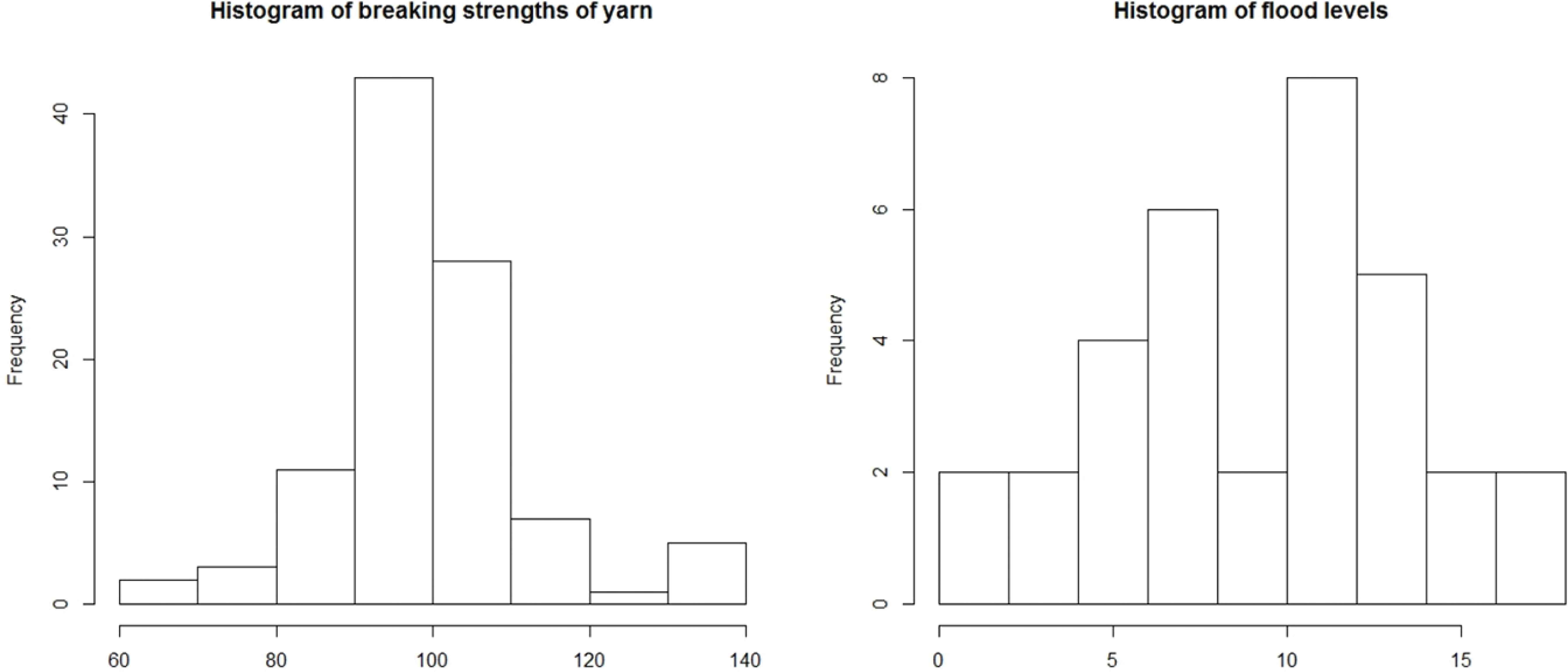
Histograms for data in Examples 1 and 2.
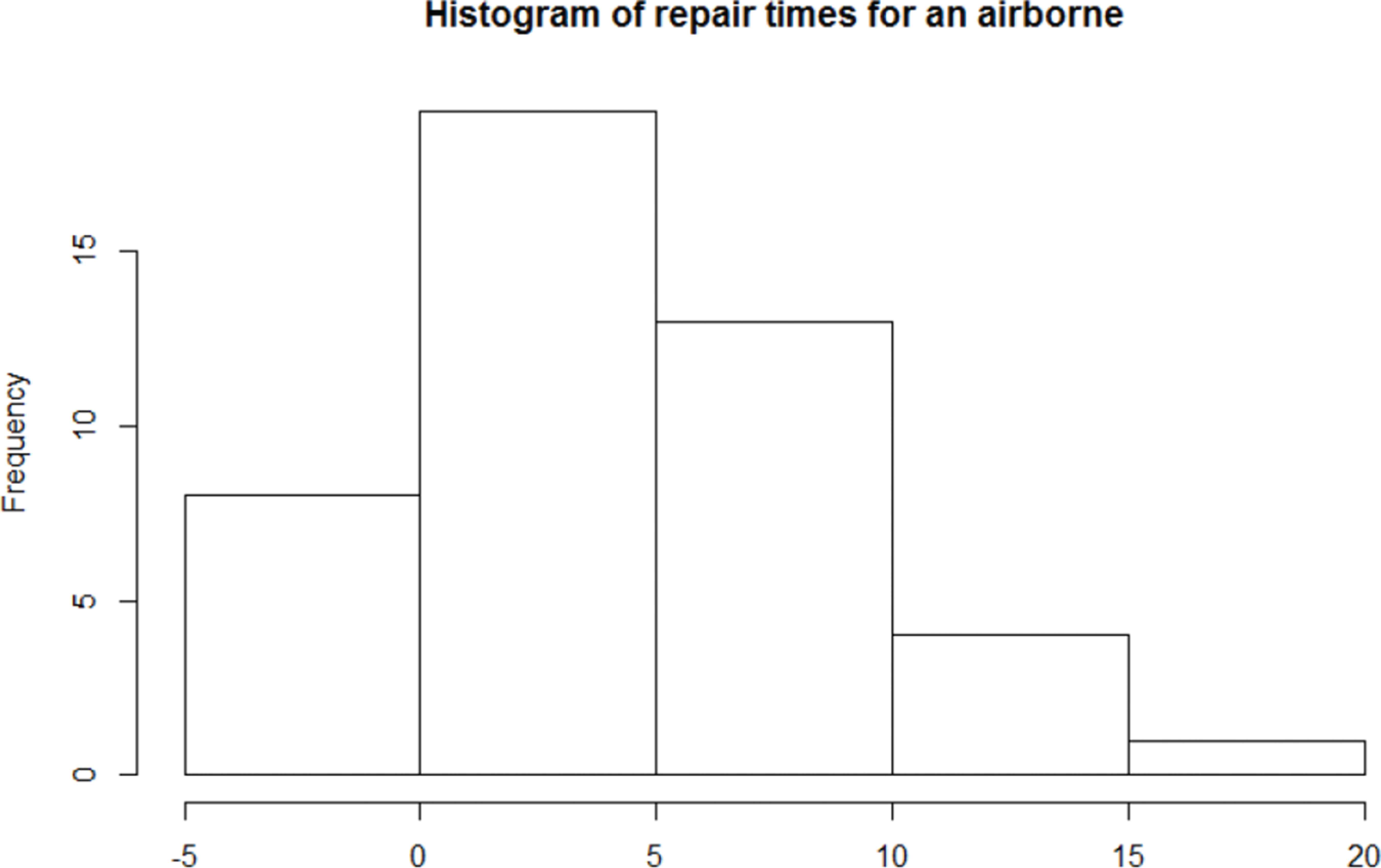
Histogram for data set in Example 3.
Example 1.
The following data are 100 breaking strengths of yarn presented by Duncan [21]:
66, 117, 132, 111, 107, 85, 89, 79, 91, 97, 138, 103, 111, 86, 78, 96, 93, 101, 102, 110, 95, 96, 88, 122, 115, 92, 137, 91, 84, 96, 97, 100, 105, 104, 137, 80, 104, 104, 106, 84, 92, 86, 104, 132, 94, 99, 102, 101, 104, 107, 99, 85, 95, 89, 102, 100, 98, 97, 104, 114, 111, 98, 99, 102, 91, 95, 111, 104, 97, 98, 102, 109, 88, 91, 103, 94, 105, 103, 96, 100, 101, 98, 97, 97, 101, 102, 98, 94, 100, 98, 99, 92, 102, 87, 99, 62, 92, 100, 96, 98.
Puig and Stephens [22] used the Empirical distribution function (EDF) tests for fitting a normal distribution for these data. They concluded that all the test statistics have significance levels below 0.01 so that the normal assumption is rejected at this level of significance.
We apply the tests for testing the assumption that the data are from a normal distribution. We obtain the maximum likelihood estimator of FMKL family as
Since
The values of the test statistics are
| Test | Value of the test statistic | p-value |
|---|---|---|
| D | 0.1569 | 0.0000 |
| V | 0.2462 | 0.0000 |
| CH | 0.4503 | 0.0000 |
| A2 | 2.7180 | 0.0000 |
| KLmn | 0.1887 | 0.0006 |
| W | 0.9904 | 0.0000 |
| JB | 31.5526 | 0.0009 |
Comparison of p-values of the tests in Example 1.
Therefore, the normal assumption is rejected by the EDF statistics. Also, the tests KLmn, W and JB reject the normal assumption.
Example 2.
Bain and Engelhardt [23] presented the following dataset, consisting of 33 difference in flood levels between stations on a river:
1.96, 1.97, 3.60, 3.80, 4.79, 5.66, 5.76, 5.78, 6.27, 6.30,6.76, 7.65, 7.84, 7.99, 8.51, 9.18, 10.13, 10.24, 10.25, 10.43, 11.45, 11.48, 11.75, 11.81, 12.34, 12.78, 13.06, 13.29, 13.98, 14.18, 14.40, 16.22, 17.06.
They suggested that the Laplace distribution might provide a good fit. Puig and Stephens [22] concluded that D and W2 reject the Laplace distribution for the data at 0.05 level and the other tests accept the Laplace assumption.
We apply the tests for testing the assumption that the data are from a normal distribution. We obtain the maximum likelihood estimator of FMKL family as
Since
The values of the test statistics are
| Test | Value of the test statistic | p-value |
|---|---|---|
| D | 0.0929 | 0.6599 |
| V | 0.1722 | 0.5707 |
| CH | 0.0416 | 0.6455 |
| A2 | 0.2467 | 0.7489 |
| KLmn | 0.2175 | 0.3734 |
| W | 0.9766 | 0.6798 |
| JB | 1.3645 | 0.3857 |
Comparison of p-values of the tests in Example 2.
Therefore, the normal assumption is accepted by all tests at the significance level of 0.05. Based on our simulation results presented in Section 3, we can accept the result obtained by KLmn test.
Example 3.
The following data represent active repair times (in hours) for an airborne communication transceiver:
0.2, 0.3, 0.5, 0.5, 0.5, 0.5, 0.6, 0.6, 0.7, 0.7, 0.7, 0.8, 0.8, 1.0, 1.0, 1.0, 1.0, 1.1, 1.3, 1.5, 1.5, 1.5, 1.5, 2.0, 2.0, 2.2, 2.5, 3.0, 3.0, 3.3, 3.3, 4.0, 4.0, 4.5, 4.7, 5.0, 5.4, 5.4, 7.0, 7.5, 8.8, 9.0, 10.3, 22.0, 24.5.
von Alven [24] fitted the lognormal distribution for these data. Chhikara and Folks [25] fitted the Inverse Gaussian (IG) distribution and justified it by the Kolmogorov–Smirnov statistic. Finally, Lee et al. [26] tested the lognormal and IG distributions which were both accepted.
We obtain the maximum likelihood estimator of FMKL family as
Since
In this case, we obtained the values of the test statistics for normal model as
| Test | Value of the test statistic | p-value |
|---|---|---|
| D | 0.2465 | 0.0000 |
| V | 0.4614 | 0.0000 |
| CH | 0.8793 | 0.0000 |
| A2 | 5.0138 | 0.0000 |
| KLmn | 0.9404 | 0.0000 |
| W | 0.6317 | 0.0000 |
| JB | 177.19 | 0.0000 |
Comparison of p-values of the tests in Example 2.
Therefore, the normal assumption is rejected by all tests at the significance level of 0.05. Based on our power study, we accept the result obtained by KLmn test.
5. CONCLUSIONS
In this paper, we considered seven popular tests for normality, namely, Kolmogorov-Smirnov, Anderson-Darling, Kuiper, Jarque-Bera, Cramer von Mises, Shapiro-Wilk and Vasicek. These tests are commonly used in practice and statistical software and therefore power values of these tests against various alternatives are important. Here, we considered the family of four-parameter GLDs which is called FMKL family, as alternatives for tests for normality.
The FMKL family is divided to five groups and therefore we computed the power values of the tests against these five groups using Monte Carlo computations for sample sizes n = 10, 20, 30 and n = 50. Differences in power of the seven tests are considerable and each of the tests JB, W and KLmn can be most powerful depending on the type of alternatives. In group I, unimodal densities with continuous tails, the tests JB and W have the most power and when
Based on these observations, we can formulate the following recommendations for the application of the tests in practice.
Use the statistics JB or W, if the assumed alternatives are in groups Ia and Ib with the exception of the cases where
Use the statistic KLmn, based on the sample entropy, if the assumed alternatives are not in groups Ia and Ib with the exception of the cases where
The author is thankful to the referees and editor-in-chief of the journal for their valuable comments and suggestions, which improved the presentation of this paper greatly.
REFERENCES
Cite this article
TY  - JOUR
AU  - Hadi Alizadeh Noughabi
PY  - 2018
DA  - 2018/12/31
TI  - A Comprehensive Study on Power of Tests for Normality
JO  - Journal of Statistical Theory and Applications
SP  - 647
EP  - 660
VL  - 17
IS  - 4
SN  - 2214-1766
UR  - https://doi.org/10.2991/jsta.2018.17.4.7
DO  - 10.2991/jsta.2018.17.4.7
ID  - Noughabi2018
ER  -