
Efficient Estimator of Parameters of a Multivariate Geometric Distribution
Corresponding author. Email: ullllhasdixit@yahoo.com.in
- DOI
- 10.2991/jsta.2018.17.4.6How to use a DOI?
- Keywords
- Multivariate geometric distribution; Maximum likelihood estimator; Uniformly minimum variance unbiased estimator; modified MLE
- Abstract
The maximum likelihood estimator (MLE) and uniformly minimum variance unbiased estimator (UMVUE) for the parameters of a multivariate geometric distribution (MGD) have been derived. A modification of the MLE estimator (modified MLE) has been derivedin which case the bias is reduced. The mean square error (MSE) of the modified MLE is less than the MSE of the MLE. Variances of the parameters and the corresponding generalized variance (GV) has been obtained. It has been shown that the MLE and modified MLE are consistent estimators. A comparison of the GVs of modified MLE and UMVUE has shown that the modified MLE is more efficient than the UMVUE. In the final section its application has been discussed with an example of actual data.
- Copyright
- © 2018 The Authors. Published by Atlantis Press SARL.
- Open Access
- This is an open access article under the CC BY-NC license (http://creativecommons.org/licences/by-nc/4.0/).
1. INTRODUCTION
It is appropriate and convenient to measure lifetime of devices such as on/off switches, bulbs, engines of an airplane on a discrete scale. Discrete random variables also help study lifetimes such as the incubation period of diseases like AIDS, the remission time of cancers as well as time to failure of engineering systems (see [1]). The discrete multivariate distributions are useful to measure lifetime data. The multivariate geometric distribution (MGD) has been vital in studying reliability analysis. Various models of the bivariate geometric distribution (BGD) have been proposed to study lifetime devices. Downtown [2] has described a model for developing a BGD. This arises in a shock model with two components. Downtown [2] describes this model asfollows. Suppose that the number of shocks suffered by each component before failure can be represented by a population in which proportions p1 and p2 affected the first and second components respectively, without failure and a proportion 1-p1-p2 of the shocks lead to failure of both the components. Hence X is number of shocks to component 1 prior to the first failure and Y is number of shocks to component 2 prior to the first failure. The joint probability function of (X, Y) is given by
The corresponding joint probability mass function of (X,Y) is
Hare Krishna and Pundir [3] have obtained the MLE and Baye’s estimators of the parameters for this BGD. Dixit and Annapurna [4] have further obtained the UMVUE estimators and have compared the MLE and UMVUE based on the mean square errors (MSEs). Phatak and Sreehari [5] introduced a version of bivariate geometric distribution as a stochastic model for giving the distribution of good and marginally good items that are produced by a production unit. Marshall and Olkin [6] constructed a BGD based on the sequence of Bernoulli random variables in which X was defined as the number of trials required for the rth occurence of an event A and Y was the number of trials required for the sth occurence of an event B. If we consider Bernoulli trials then (X,Y) will have 4 possible values (0,0), (0,1), (1,0) and (1,1).
We define
Let
The marginal probability functions are of the usual form but the joint probability function of (X,Y) is quite complicated. Reference may be made to Marshall and Olkin ([6], Eq. 7.2).
On the same lines, Gultekin and Bairamov [7] constructed a trivariate geometric distribution and the corresponding multivariate extension. Srivastava and Bagchi [8] introduced the multivariate version of a geometric distribution and obtained certain characterizations. Vasudeva and Srilakshminarayana [9] established some properties of the MGD and also obtained a characterization assuming it to follow the power series distribution. Sreehari and Vasudeva [10] have given characterization of the MGD based on conditional distributions. Esary and Daniel [11] studied properties of MGDs that were generated by a cumulative damage process. In this paper we look at another form of the MGD and estimate its parameters by a new approach that reduces the bias.
Consider a system which comprises of k components namely C1,C2,…,Ck. The system is so designed that at any given time not more than one component can function. The system functions when any one component functions. The system initially functions because C1 functions. When C1 stops functioning C2 starts functioning in the next trial keeping the system functioning. Thus system continues to function in this manner till Ck functions. Let probability that component Ci fails be pi, i = 1,2,3, …, k. Let Xi denote the trial at which component Ci fails, i = 1,2, …, k.
The joint probability mass function of (X1,X2, …, Xk) is given as
The probability generating function (pgf) is given as
In this paper we obtain UMVUE and MLE of the parameters in Eq. (1) and their functions.
2. UNIFORM MINIMUM VARIANCE UNBIASED ESTIMATOR (UMVUE)
Here we obtain the UMVUE of the parameters as well as of the functions of the parameters. We consider the trivariate case which has three parameters, p1, p2 and p3. Here pi denotes the corresponding probability of the ith component in the system failing.
Consider the case where k = 3. Eqs. (1) and (2) become
The pgf of
Hence the pmf of S1, S2 and S3 is co-efficient of
Theorem 2.1.
The UMVUE of
Proof.
The trivariate joint distribution of
Let
Hence
Therefore
Particular Cases
Similarly it is possible to obtain UMVUE for various combinations of
Theorem 2.2.
The UMVUE in the multivariate case of
3. MAXIMUM LIKELIHOOD ESTIMATOR (MLE)
In the earlier section we have obtained an estimator based on the criteria of unbiasedness and minimum variance. We now look at another very popular principle used namely method of maximum likelihood to obtain the estimators of the functions of the parameters. These shall be compared with the corresponding estimators obtained by UMVUE in order to study their efficiency. The likelihood function based on n systems put on test strictly under the same conditions will be
Taking log and differentiating w.r.t pi, i = 1,2, …, k, the MLEs are obtained as
The MLE of pi; i = 1,2,. …, k is
By invariance property, MLE of
4. MODIFIED MAXIMUM LIKELIHOOD ESTIMATOR (MODIFIED MLE)
In the earlier two sections we have applied two procedures to obtain the estimators and either of them could be good. We now try to improve on the MLE by reducing the bias and thus derive a modified estimator namely modified MLE. We have further shown thatthis modified MLE is better than the UMVUE. Hence to derive a modification that reduces the bias and the MSE of the MLE of pi, i = 1,2,3, …, k, we apply the Taylor Series two-parameter expansion to
On substition of Eqs. (21) in (22) we obtain
On taking expectaion of Eq. (24) we obtain
We observe that
Consider a linear function of the MLE of pi given as
Hence
If the coefficient of pi is set equal to 1 and the constant term set equal to zero, we obtain aproximate equality between
This gives us
Therefore we obtain a modified MLE of pi
Since
Thus
Thus the MSE of modified MLE of
5. CONSISTENCY OF MODIFIED MLE
If we collect a large number of observations, then we can obtain a lot of information about the unknown parameter. We can thus construct an estimator T(X) with a small MSE and we can call it a consistent estimator if
Theorem 5.1.
Proof.
From Eq. (25) it is clear that
Let k = 1
Applying the Taylor series expansion
On taking expectaion of
Hence
Thus
Consider k = 2
Here
Applying Taylor Series two parameter expansion we obtain
Hence
Assume
To prove that
We need to prove that
To obtain
Thus as n tends to ∞,
We now consider
Thus from Eq. (39) and since
But
The
Thus, since
Note: The MSE of modified MLE is less than MSE of MLE from Eq. (29).
From Eq. (28) we can conclude that the modified MLE,
6. CONCLUSION AND COMPARISION OF ESTIMATORS
We have observed in the earlier section that an improvement over the MLE is the modified MLE. We now have two estimators the UMVUE and the modified MLE. Our objective is to compare both the estimators with respect to efficiency. We make a comparative study of the two based on the determinant of the variance covariance matrix also called as the generalised variance (GV). We consider the trivariate case namely k = 3. The variances and covariances of the UMVUE and modified MLE of the parameters can be obtained as below. Consider the case when k = 3.
Variance of UMVUE of pi, i = 1, 2, 3 where
Covariance of the UMVUEs of pi and pj, i, j = 1, 2, 3 and
Variance of modified MLE of pi when k = 3 is
Covariance of modified MLE of pi and pj, i, j = 1, 2, 3 and
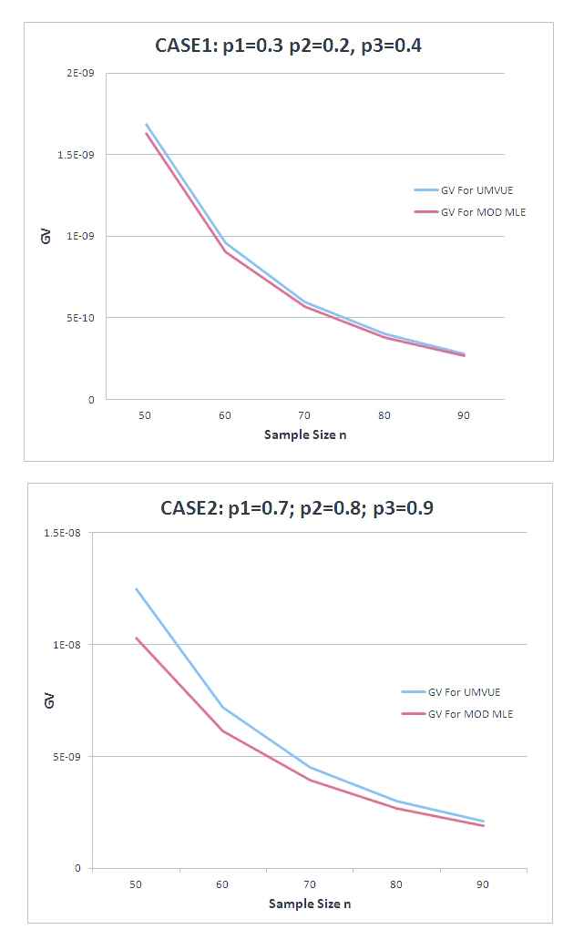
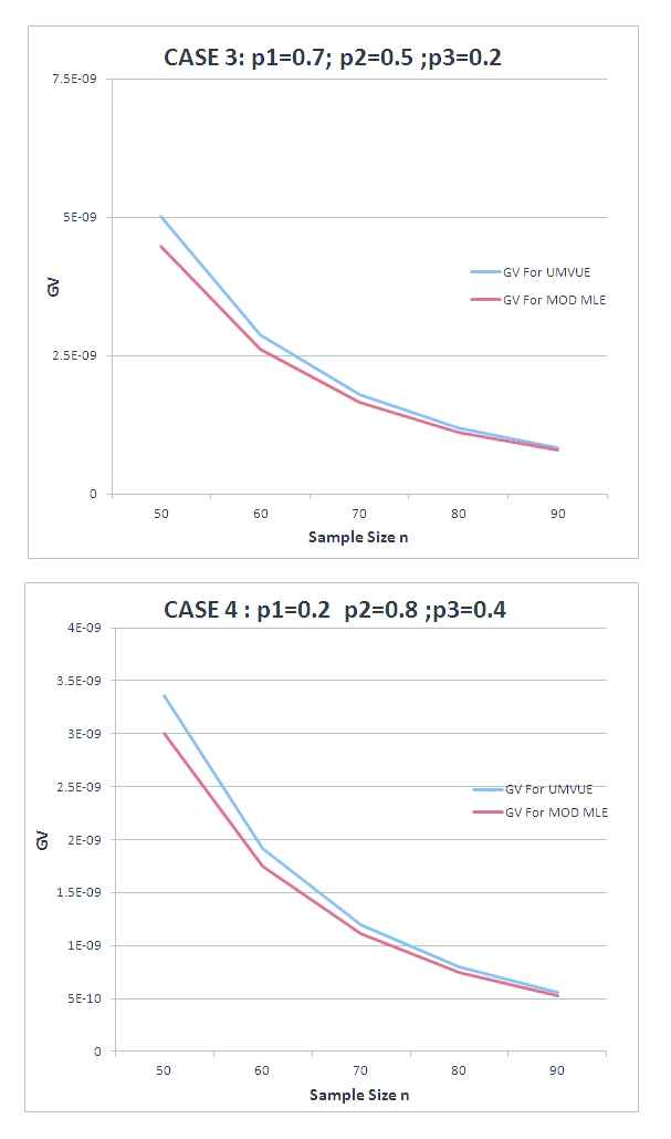
The determinant of the variance covariance matrix is calculated and are compared for the two estimators in the graphs below for a range of values of the parameters p1, p2 and p3.
It can be observed from the graphs in Figs. 1 and 2 that the generalised variance of the modified MLE is less than the corresponding GV of the UMVUE for numerical values of p1, p2 and p3 ranging from 0.1 to 0.9. Thus we obtain a new and better estimator called modified MLE which is consistent. It is an improvement over the MLE and is also more efficient than the UMVUE.
The generalised variance of the modified MLE
The generalised variance of the modified MLE
7. AN EXAMPLE FOR k = 3
A game of cricket has been considered. When a batsman is out he is replaced by another batsman in the next ball and the game continues. When the replaced batsman is declared out another replacement is sent forth and the game continues. Consider the 2016 season of Cricket's Indian Premium League ‘IPL 2016’. A total of 17 matches were played by the winning team. Sunrisers Hyderabad, of which 15 were suitable for our study. We have recorded the following details.
Let
Xi denote the ball at which the first player becomes out in the ith match.
Yi denote the ball at which the player who replaces the first batsman becomes out in the ith match.
Zi denote the ball at which the player who replaces the second batsman becomes out in the ith match, i = 1, 2, …, 15.
| Match No i | Xi | Yi | Zi |
|---|---|---|---|
| 1 | 25 | 29 | 35 |
| 2 | 7 | 16 | 27 |
| 3 | 4 | 26 | 38 |
| 4 | 31 | 32 | 52 |
| 5 | 4 | 18 | 20 |
| 6 | 11 | 49 | 52 |
| 7 | 17 | 26 | 42 |
| 8 | 33 | 38 | 61 |
| 9 | 14 | 51 | 56 |
| 10 | 30 | 54 | 56 |
| 11 | 8 | 9 | 20 |
| 12 | 16 | 41 | 50 |
| 13 | 10 | 31 | 61 |
| 14 | 4 | 10 | 23 |
| 15 | 25 | 30 | 53 |
IPL 2016: Team Hyderabad Sunrisers
Hence
Thus for n = 15, we obtain s1 = 239, s2 = 460 and s3 = 646. The MLE, UMVUE and modified MLE for the following parameters are as shown in Table 2.
| P1 | P2 | P3 | |
| UMVUE | 0.05882 | 0.063636 | 0.075676 |
| MLE | 0.06276 | 0.06787 | 0.0806 |
| Modified MLE | 0.05884 | 0.063631 | 0.075605 |
Values of MLE, UMVUE and modified MLE for parameters
From the example of IPL2016, it is observed that the UMVUE, MLE and modified MLE estimates calculated for p1, p2 and p3 are very close to each other.
ACKNOWLEDGEMENT
We are thankful to the referees and the editor for their valuable comments and constructive suggestions which has improved this manuscript.
REFERENCES
Cite this article
TY  - JOUR
AU  - U. J. Dixit
AU  - S. Annapurna
PY  - 2018
DA  - 2018/12/31
TI  - Efficient Estimator of Parameters of a Multivariate Geometric Distribution
JO  - Journal of Statistical Theory and Applications
SP  - 636
EP  - 646
VL  - 17
IS  - 4
SN  - 2214-1766
UR  - https://doi.org/10.2991/jsta.2018.17.4.6
DO  - 10.2991/jsta.2018.17.4.6
ID  - Dixit2018
ER  -