
Interval-valued uncertainty based on entropy and Dempster–Shafer theory
Corresponding author. Emails: pashaeinollah@yahoo.com; pasha@khu.ac.ir
- DOI
- 10.2991/jsta.2018.17.4.5How to use a DOI?
- Keywords
- Epistemic uncertainty; Aleatory uncertainty; Shannon entropy; Dempster–Shafer theory; Upper and lower bounds
- Abstract
This paper presents a new structure as a simple method at two uncertainties (i.e., aleatory and epistemic) that result from variabilities inherent in nature and a lack of knowledge. Aleatory and epistemic uncertainties use the concept of the entropy and Dempster–Shafer (D–S) theory, respectively. Accordingly, we propose the generalized Shannon entropy in the D–S theory as a measure of uncertainty. This theory has been originated in the work of Dempster on the use of probabilities with upper and lower bounds. We describe the framework of our approach to assess upper and lower uncertainty bounds for each state of a system. In this process, the uncertainty bound is calculated with the generalized Shannon entropy in the D–S theory in different states of these systems. The probabilities of each state are interval values. In the current study, the effect of epistemic uncertainty is considered between events with respect to the non-probabilistic method (e.g., D–S theory) and the aleatory uncertainty is evaluated by using an entropy index over probability distributions through interval-valued bounds. Therefore, identification of total uncertainties shows the efficiency of uncertainty quantification.
- Copyright
- © 2018 The Authors. Published by Atlantis Press SARL.
- Open Access
- This is an open access article under the CC BY-NC license (http://creativecommons.org/licences/by-nc/4.0/).
1. INTRODUCTION
Several mathematical frameworks can be used to evaluate an uncertainty analysis. Probability theory is the most traditional representation of uncertainty, which is familiar to non-mathematicians. Probability is used as a representation of subjective belief, which is common in a quantitative analysis of events in different applications. Safety assessments should deal with rare events, and thus it is difficult to assess the relative frequencies of these events [1]. The Bayesian approach for the uncertainty analysis is to specify a coherent probability measure as the current state of available knowledge and uses Bayes’ theorem to adjust the probabilities as new evidence, which is unveiled. Though Bayesian inference can be employed to determine the probability of decisions correctness based on prior information, it has some disadvantages, namely (1) the knowledge required to generate the prior probability distributions may not be available, (2) instabilities may occur when conflicting data are presented and/or the number of unknown propositions is large compared to the known propositions [2], (3) available information should be characterized by a specific distribution or an exact assertion of the truth of a proposition for the decision maker, and (4) Bayesian inference offers a few opportunities to express incomplete information or partial belief [3].
Imprecise probability is a generic term for any mathematical model, which measures chance or uncertainty without crisp numerical probabilities. The evidence or Dempster–Shafer (D–S) theory of belief structures is one type of imprecise probabilities, which offers a more flexible representation of uncertainty over the crisp probabilistic approach. Based on the Dempster's work, Shafer [4] proposed the D–S theory as an alternative to Bayesian inference. This theory is a generalization of the Bayesian theory and can robustly deal with incomplete data. It allows the representation of both imprecision and uncertainty [5, 6]. Rather than computing probabilities of propositions, it computes probabilities that evidence supports the propositions or alternatives, which deal with uncertainty reasoning based on incomplete information. The D–S theory tackles the prior probability issue by keeping a track of an explicit probabilistic measure of a possible lack of information. It is suitable for taking into account the disparity among knowledge types [7]. Because it is able to provide a federative framework [8] and combines cumulative evidence for changing prior opinions in the light of new evidence [9].
The D–S theory is well developed and considered as the most appropriate alternative for uncertainty quantification, which deals with lack of knowledge. For example, Jiang et al. [10] proposed a new method to deal with a reliability analysis to solve engineering problems by using the D–S theory under uncertainty. Tang et al. [11] presented an evidential uncertainty quantification method to determine uncertainties with imprecise information, which is included in revealing the material constants of the metal fatigue crack growth model. Yin et al. [12] proposed an efficient algorithm to solve an acoustic problem under uncertainty and applied the Jacobi polynomial for evidence-theory based on an uncertainty analysis. Then, Yin et al. [13] analyzed the response of built-up systems in the mid-frequency range by using the D–S theory and a model of a finite element/statistical energy analysis under uncertainty. Jian et al. [14] evaluated flutter risk and the structural stability of the system, which deals with the D–S theory and uncertainty quantification.
In the probability theory, Shannon entropy is one of the best-known measures of uncertainty for a purely probabilistic system [15]. Based on the Shannon entropy concept, many studies have formulated to handle uncertainty in different fields of science. For example, Thapliyal and Taneja [16] used the concept of the Shannon entropy to evaluate the uncertainty as a measure of inaccuracy associated with distributions of order statistics. Olvera-Guerrero et al. [17] used the non-linear Shannon entropy to measure the uncertainty of a boiling water reactor to assess a system stability and operation.
Gu [18] introduced a new concept of entropy and multi-scale Shannon entropy and then analyzed its application to detect predictive power for the Dow Jones Industrial Average Index (DJIAI). In the fields of component lifetimes of a system, Gupta et al. [19] considered the Shannon entropy as a measure of the uncertainty associated with a residual lifetime distribution and acquired the properties of the residual and the entropy function of order statistics. Tahmasebi et al. [20] proposed a new extension of cumulative residual entropy using the Shannon entropy as a measure of the uncertainty associated with the lifetime of a system. Toomaj and Doostparast [21] introduced a new concept of a stochastic order for comparing mixed systems and used cumulative residual entropy, which measures the residual uncertainty of a random variable. They applied these concepts to evaluate component lifetimes of competing systems using the Shannon entropy, in order to handle uncertainty. The other applications are fault diagnosis [22], risk [23], etc.
Generally, frameworks, which are considered the uncertainty of the physical events or the behavior of a system, can be categorized into two types of uncertainty. Type one is uncertainty due to stochastic and irreducible variabilities, which is inherent in nature (i.e., aleatory uncertainty), and the other one is resulting from unknown physical phenomena due to a lack of knowledge (i.e., epistemic uncertainty). In Section 2, a brief introduction is provided two uncertainties. For adequate data existing in probability theory, numerous uncertain models (e.g., various types of entropies) are used as the most appropriate evaluation for aleatory uncertainty quantification. Non-probabilistic methods based on interval specifications or alternative mathematical frameworks (e.g., D–S theory) are proposed for possible better representations of epistemic uncertainty.
Obviously, in the analysis process of the system performance, uncertainty appears at different steps of analysis and the interaction between these sources of uncertainty cannot be modeled easily. Thus, in order to evaluate and reduce uncertainty, different models and modern mathematical frameworks have been proposed to quantify both aleatory and epistemic uncertainties in systems (e.g., see [24, 25]). However, the existing methods to evaluate the effect of mixed uncertainty using a piece of information and different mathematical frameworks are efficient, and modern frameworks for mathematical representation of uncertainty are still under development.
Therefore, in this paper, the concepts of D–S theory and Shannon entropy are used to handle uncertainty for systems’ failure in each state considering the uncertainty bounds. On the other hand, the objective is to introduce a new technique to calculate uncertainty bounds based on the D–S theory and Shannon entropy. This paper is organized as follows. In Section 2, we introduce the type of uncertainty. Sections 3 and 4 introduce some concepts of the D–S theory and Shannon entropy as a measure of uncertainty. Section 5 describes a heuristic method for the entropy of interval-valued probabilities. It is assumed that there is a system with n different states. Conclusions are summarized in Section 6.
2. TYPES OF UNCERTAINTY
In the field of uncertainty quantification, uncertainty in the governing equations may assume two uncertainties (i.e., aleatory and epistemic). Aleatory uncertainty can be characterized by known probability distributions whilst epistemic uncertainty arises from a lack of knowledge of probabilistic information. It arises from the inherent variation associated with the system under consideration and is irreducible. The sources of aleatory uncertainty are typically represented by using a probabilistic framework. It is referred to inherent uncertainty due to the attribute of intrinsic randomness and probabilistic variables, which is associated with the physical system.
On the other hand, it is a result of a naturally occurring process, variability in the underlying variables or statistical variability, which is stochastic and more collected data in a given model cannot reduce this uncertainty. Thus, stochastic uncertainty in the sequence of possible events is entirely aleatory by nature. Epistemic uncertainty represents any lack of knowledge or information in any phase or activity of the modeling process [26, 27] and it is reducible through the introduction of additional information. Source of this uncertainty is of data completeness and quality. Hence, it can be reduced by more knowledge that is available. Therefore, epistemic uncertainty is reducible as results of an inaccurate scientific understanding of the natural phenomenon being modeled or data quality, completeness or incomplete knowledge of the underlying process.
Frequently, strong statistical information (e.g., probability distribution functions or high-order statistical moments) is not available. Experimental data needed to construct this information are often expensive. Thus no data or only a small collection of data points may be obtainable consequently. In these cases, expert opinion is used to handle epistemic uncertainty in conjunction with the available data to produce weak inferential estimates of parametric characteristics in a form of lower and upper bounds.
Other sources of epistemic uncertainty include limited understanding or misrepresentation of a modeled process, known commonly as a model specification uncertainty. The inclusion of enough additional information about either the model parameters or structure can lead to a reduction in the predicted uncertainty of a model output. Consequently, we can consider epistemic uncertainty as providing (conservative) bounds on an underlying aleatory uncertainty, in which reduction and convergence to the true aleatory uncertainty (or a constant value in some cases) can be obtained given sufficient additional information [28]. To learn more, the reader may find some information about evidence theory [25, 29], possibility theory [30], interval analysis [31], discrete probability distributions [32], fuzzy arithmetic [33] and probability bounds [34, 35]. These theories are different from each other in terms of characterizing the input parameter uncertainty and kind of propagation from a parameter level to model an output level. In this paper, we propose a framework for quantification of epistemic uncertainty. We calculate the upper and lower bounds for uncertainty based on entropy and D–S theory.
3. D–S THEORY OF EVIDENCE
The D–S theory is a mathematical theory of evidence first proposed by Dempster in early 1967 and then extended by Shafter in 1976. It makes inferences based on uncertain knowledge from different information sources. This theory allows strengthening or erosion of beliefs by combining additional sources of evidence, even in the presence of partly contradictory evidence. There are three critical functions in the D–S theory, namely the basic probability assignment function (BPA or m), the belief function (Bel), and the plausibility function (Pl). For a finite set of mutually exclusive and exhaustive propositions (i.e., Ω), a power set 2Ω is the set of all the subsets of Ω including itself and a null set ∅. The basic probability assignment is a critical variable of evidence theory and does not refer to probability in the classical sense. For any subset A of 2Ω, the BPA, represented as m(A), defines a mapping of 2Ω to the interval between 0 and 1. Formally, this description of. can be represented by:
The upper and lower bounds of an interval can be defined from the BPA. This probability interval contains the precise probability of a set of interest in the classical sense and is bounded by two measures, namely Bel and Pl. The lower bound Bel for a set A is defined as the sum of all the BPAs of the proper subsets (B) of the set of interest (A) (
It is readily provable that Bel and Pl have the following relation.
Example 1:
Assuming
Example 2:
Assume that a system's failure states include a, b, and c. The fault hypothesis set is
Therefore, we have:
By applying the D–S theory of combination on sources of information A and B, the following data are generated based on these evidence sources as summarized in Table 1. The results are as follows.
| {a} 0.0 | {ϕ} 0.0 | {ϕ} 0.0 | {a} 0.0 | {a} 0.0 | {ϕ} 0.0 | {a} 0.0 | |
| {ϕ} 0.28 | {b} 0.0 | {ϕ} 0.0 | {b} 0.0 | {ϕ} 0.0 | {b} 0.0 | {b} 0.0 | |
| {ϕ} 0.0 | {ϕ} 0.0 | {c} 0.0 | {ϕ} 0.0 | {c} 0.0 | {c} 0.0 | {c} 0.0 | |
| {a} 0.0 | {b} 0.0 | {ϕ} 0.0 | {a, b} 0.0 | {a} 0.0 | {b} 0.0 | {a, b} 0.0 | |
| {a} 0.0 | {ϕ} 0.0 | {c} 0.0 | {a} 0.0 | {a, c} 0.0 | {c} 0.0 | {a, c} 0.0 | |
| {ϕ} 0.14 | {b} 0.0 | {c} 0.0 | {b} 0.04 | {c} 0.0 | {b, c} 0.0 | {a, c} 0.02 | |
| {a} 0.28 | {b} 0.0 | {c} 0.0 | {a, b} 0.08 | {a, c} 0.0 | {b, c} 0.0 | Ω = 0.04 |
Combination of information A and B.
Similarly, belief and plausibility functions and belief interval can be determined by using the corresponding equation described earlier, as shown in Table 2. By combining m(A) with m(B) using Eqs. (7) and (8), a new BPA m(C) characterized for all the contain subsets. Table 2 represents BPA (or mass function), belief, plausibility, belief interval and uncertainty value of the subsets. Belief intervals allow reasoning about the certainty of our beliefs or the degree of certainty. Accordingly, small differences between belief and plausibility show less certainty about our belief. Conversely, large differences show the more uncertainty about our belief.
| subsets | m(C) | bel(C) | pl(C) | belief interval | |
|---|---|---|---|---|---|
| ∅ | 0.0 | 0.0 | 1.0 | [0.0, 1.0] | 0.0 |
| {a} | 0.48 | 0.48 | 0.67 | [0.48, 0.67] | 0.19 |
| {b} | 0.27 | 0.27 | 0.49 | [0.27, 0.49] | 0.22 |
| {c} | 0.0 | 0.0 | 0.09 | [0.0, 0.09] | 0.09 |
| {a, b} | 0.13 | 0.88 | 0.97 | [0.88, 0.97] | 0.09 |
| {a, c} | 0.0 | 0.48 | 0.7 | [0.48, 0.7] | 0.22 |
| {b, c} | 0.03 | 0.3 | 0.49 | [0.3, 0.49] | 0.19 |
| Ω | 0.06 | 1.0 | 1.0 | [1.0, 1.0] | 0.0 |
Interval-valued uncertainty.
The probability in each subset lies somewhere between belief and plausibility values. A belief function represents the evidence or information, which is supported by each subset directly. Thus, the probability cannot be less than this value. A plausibility function represents an upper bound on the degree of support that can be assigned to each subset if more specific information becomes available. It is the maximum share of the evidence, which can possibly have for all subsets. Therefore, a plausibility function is the maximum possible value of probability.
In this example, comparing the impact of the uncertainty about each subset with other uncertainties shows that, in states c ({c}) and a or b ({a, b}), it is the lowest uncertainty bound (expect of Ω and ∅) between all uncertainty bounds. It is equal to 0.09, while the belief degree on states a or b ({a, b}) is the highest one (i.e., 0.88). On the other hand, with the minimum uncertainty, the most likely fault or failure occur in states a or b. Therefore, based on evidence from two samples, state a or b has the highest probable value of event on the system behavior. Although, a determination of a fault state in this example is obvious and simple; however, Eq. (9) may generally be considered as a comparison index to express relations between subsets using belief intervals [37], which will have a similar result based on the above reasons.
4. SHANNON ENTROPY
Shannon [15] presented entropy as a measurement of the uncertainty level of information. The entropy is a function of the probability distribution function. Let x be a nominal attribute on a finite set
The Shannon entropy can be taken as a measure of the uncertainty about the realization of a random variable. Entropy has the following properties: (1) by convention,
5. ENTROPY AND INTERVAL-VALUED PROBABILITY
Uncertainty is usually related to lack of knowledge about future events. Thus, a definition of risk can be considered as the amount of lacking information. Therefore, in this approach, we adopt the idea that uncertainty reflects how much we do not know about the future. Entropy is the basic notion in the information theory field. Informally, we can define entropy as the measure of uncertainty of a system that at a given moment can be in one of n states, in which a set of all the possible states is defined, and the probability of some system states is known. We can define entropy formally as follows.
Let us assume that there are n different states, where a system can be in
If values of all Pi in Eq. (11) are known, then the entropy of a system can be calculated by:
Let us consider how the entropy can be calculated if we are dealing with the interval-valued probability values. Obviously, the entropy itself will be interval-valued. In this section, we introduce a generalized definition of entropy, suitable for interval-valued probabilities. As before, we assume that system can be in n states; however, the probability that a system is in the i-th state is the interval and is equal to
If probabilities are interval-valued, then this constraint can be rewritten by:
It is easy to show that Eq. (13) is a special case of Eq. (14), when
It should be noted that the states with lower probability values are more informative. Thus, we can expect that in order to calculate the upper boundary of entropy Hmax, we should use the lower probability bounds Beli. We can find the upper boundary of entropy for a system by:
Example 3:
Assume that three information sources A, B and C are under consideration with different states (e.g.,
The uncertainty interval in the case at hand is as follows:
Therefore, it can be noticed that based on evidence from three samples, the uncertainty interval for the system's failure in state a is [0.13, 0.24].
From Eq. (16), it follows that
The obtained definition of this interval-valued probability is a generalization of the “traditional” entropy of a system with single-valued probabilities (or mass function). Now let us examine whether the additivity feature holds for the generalized entropy in the D–S theory, as defined in Eqs. (17) and (18). If additivity holds, it means whether we have two independent systems (say, X and Y), then entropy based on the D–S theory of a system obtained by joining systems X and Y is equal to the sum of individual generalized entropies in the D–S theory for X and Y. In other words, if additivity holds, then we have:
If we define generalized entropy in the D–S theory as Eqs. (17) and (18), then it can be shown that we have two systems (i.e., X and Y) with states accordingly
Therefore, we can determine the approximate uncertainty bounds (i.e., lower and upper uncertainty bounds) of two independent systems that should be summed separately to obtain the corresponding bounds of each system. These values from each interval contribute to Hmin and Hmax are shown in Fig. 1.
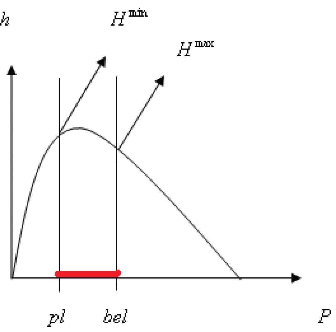
Upper and lower bounds of uncertainty.
In addition, the relative entropy is another important concept of entropy. It is known as a measure of distance between two probability distributions. It is evaluated divergence between probabilities or mass function of two systems
Let
Obviously, if and only if
Furthermore, the lower bound for the relative entropy with respect to plausibility functions
6. CONCLUSION
One way to assess the uncertainty between proposed theories under imprecise probabilities is the D–S theory. In probability theory, the best-known measure of uncertainty in a purely probabilistic system is the Shannon's entropy. This paper incorporates information and probabilities for different states of systems considered as an interval-valued probability, and then a heuristic approach is used to generalize entropy in the D–S theory for an uncertainty model. This approach is proposed to approximate upper and lower uncertainties for a presented formal problem. Since it is hard to solve this formal problem directly, the proposed method is a proper method to find an approximate solution. Accordingly, different examples are presented for the simple proposed method. The results show the efficiency of the method to find an approximate solution to quantify uncertainty bounds. Furthermore, the new definition of uncertainty bounds for two independent systems is explained, which is held by the additivity property. Then, quasi-additivity of uncertainty bounds is shown in Fig. 1. Finally, the upper and lower bounds of relative entropy are presented to evaluate the divergence between two mass functions.
ACKNOWLEDGEMENTS
The authors would like to thank the Editor-in-Chief and autonomous reviewers for their constructive comments and helpful suggestions, which greatly improved the presentation of this paper.
REFERENCES
Cite this article
TY  - JOUR
AU  - F. Khalaj
AU  - E. Pasha
AU  - R. Tavakkoli-Moghaddam
AU  - M. Khalaj
PY  - 2018
DA  - 2018/12/31
TI  - Interval-Valued Uncertainty Based on Entropy and Dempster–Shafer Theory
JO  - Journal of Statistical Theory and Applications
SP  - 627
EP  - 635
VL  - 17
IS  - 4
SN  - 2214-1766
UR  - https://doi.org/10.2991/jsta.2018.17.4.5
DO  - 10.2991/jsta.2018.17.4.5
ID  - Khalaj2018
ER  -