Journal of Statistical Theory and Applications

Volume 18, Issue 1, March 2019, Pages 33 - 45

Discrete Additive Weibull Geometric Distribution

Authors
K. Jayakumar1, M. Girish Babu2, *
1Department of Statistics, University of Calicut, Malappuram, Kerala-673 635, India
2Department of Statistics, Government Arts and Science College, Meenchanda, Kozhikode, Kerala-673 018, India
*Corresponding author. Email: giristat@gmail.com
Corresponding Author
M. Girish Babu
Received 2 August 2017, Accepted 13 February 2018, Available Online 22 April 2019.
DOI
10.2991/jsta.d.190306.005How to use a DOI?
Keywords
Additive Weibull distribution; discrete Weibull distribution; geometric distribution; hazard rate function; order statistics; Weibull distribution
Abstract

Discretizing a continuous distribution has received much attention among researchers recently. Discrete analogue of the well-known continuous distributions such as Normal, Exponential, Weibull, Laplace, Rayleigh, and so on, are available in the literature. In this paper, we introduce a discrete version of the additive Weibull geometric distribution of Elbatal et al. [1]. Discrete Weibull, discrete modified Weibull, discrete Weibull geometric, discrete exponential geometric, discrete Rayleigh distribution, and so on, are sub models of this distribution. We study some properties of the new distribution. The hazard rate function of the new distribution is monotonically increasing or decreasing or bathtub shape based on the values of the shape parameters. The method of maximum likelihood estimation is used for estimating the model parameters. A simulation study is carried out to show the performance of the maximum likelihood estimate of parameters of the new distribution. An application of this distribution to a real data set is also presented.

Copyright
© 2019 The Authors. Published by Atlantis Press SARL.
Open Access
This is an open access article distributed under the CC BY-NC 4.0 license (http://creativecommons.org/licenses/by-nc/4.0/).

1. INTRODUCTION

There are situations where continuous random variables may not necessarily always be measured on a continuous scale but may often be counted as discrete random variable. For example, in military service, the weapons like tanks, what is more important is the number of times it fires until failure than the life of the weapon. Similar situations frequently occur in reliability and survival analysis. By discretizing the continuous distribution, several discrete lifetime distributions are developed in the literature. Some of them are discrete Weibull distribution in Nakagawa and Osaki [2], a second type of discrete Weibull distribution in Stein and Dattero [3], a third type of discrete Weibull distribution in Padgett and Spurrier [4], discrete exponential distribution in Sato et al. [5], discrete normal distribution in Roy [6], discrete Rayleigh distribution in Roy [7], discrete Laplace distribution in Inusah and Kozubowski [8], discrete skew-Laplace distribution in Kozubowski and Inusah [9], discrete Burr and discrete Pareto distributions in Krishna and Pundir [10], discrete inverse Weibull distribution in Jazi et al. [11], discrete generalized exponential distribution in Gómez-Déniz [12], discrete generalized exponential distribution in Nekoukhou et al. [13], discrete gamma distribution in Chakraborty and Chakravarty [14], discrete additive Weibull (AW) distribution in Bebbington et al. [15], discrete Lindley distribution in Bakouch et al. [16], discrete Gumbel distribution in Chakraborty and Chakravarty [17], exponentiated geometric distribution in Chakraborty and Gupta [18], discrete distribution related to generalized gamma distribution in Chakraborty [19], transmuted geometric distribution in Chakraborty and Bhati [20], discrete Weibull geometric (DWG) distribution in Jayakumar and Babu [21], and so on.

Discretization plays a vital role in variable selection method, in addition to transforming the continuous variable to discrete variable. This method can significantly make an impact on the performance of classification algorithms applied in the analysis of high-dimensional biomedical data. While constructing the discrete version of a continuous distribution, one may preserve one or more characteristic properties of the continuous one. There are different methodologies available in the literature about the discretization of a continuous distribution (see Bracquemond and Gaudoin [22], Chakraborty [23]).

Discretization of the distribution of a continuous random variable X, to its discrete analogue, say Y, using the method of survival functions is given by

PY=y=PX≥y−PX≥y+1=SXy−SXy+1; y=0,1,2, … ,
where, Y=[X]= largest integer less than or equal to X and SX. is the survival function of the random variable X.

Xie and Lai [24] proposed the AW distribution by combining the failure rates of two Weibull distributions of which one has a decreasing failure rate and the other has an increasing failure rate. The cumulative distribution function (cdf) of AW distribution is given by

Fx;α,β,γ,δ=1−e−αxβ+γxδ,
where α>0,γ>0 and β>δ>0 or (δ>β>0), which gives identifiability to the model. Here α and γ are scale parameters, and β and δ are shape parameters. Lemonte et al. [25] examined some structural properties of AW distribution.

Suppose X1,X2,…,XN are N independent and identically distributed (iid) random variables from AW distribution with cdf given in Eq. (2). Let N be a discrete random variable following geometric distribution (truncated at zero) with probability mass function (pmf) given by

PN=n=1−ppn−1; n=1,2,…;0<p<1.

Let X1=MinXii=1N. Then the cdf of X1|N=n, is given by,

GX1|N=nx=1−1−Fxn=1−e−nαxβ+γxδ.

Hence, the cdf of X1 is

Fx;α,β,γ,δ,p=1−p∑n=1∞pn−11−e−nαxβ+γxδ=1−e−αxβ+γxδ1−pe−αxβ+γxδ,
where x>0, 0<p<1, α>0, β>0, γ>0 and δ>0. The distribution of X1 is called AW geometric and its survival function is given by,
Sx;α,β,γ,δ,p=1−pe−αxβ+γxδ1−pe−αxβ+γxδ

This distribution is studied by Elbatal et al. [1].

The contents of the paper are arranged as follows: In Section 2, the discrete AW geometric (DAWG) distribution is introduced and in Section 3, various properties of this distribution including the structure of hazard rate function are studied. In Section 4, the maximum likelihood estimation (MLE) method is used for parameter estimation. Also a simulation study is carried out to study the performance of the maximum likelihood estimates of the new distribution. Application of this distribution in real data modeling is illustrated in Section 5 and conclusions are presented in Section 6.

2. DAWG DISTRIBUTION

Marshall and Olkin [26] introduced a method of adding a parameter into a family of distributions. According to them if F¯x denote the survival function of a continuous random variable X, then the usual device of adding a new parameter results in another survival function G¯x is defined by

G¯x=θF¯x1−θ¯F¯x ,−∞<x<∞, θ>0,
where θ¯=1−θ. In particular when θ=1, G¯x=F¯x.

Let Y be the discrete analogue of the continuous random variable X with survival function defined in Eq. (7). Gómez-Déniz [12] obtained the discrete analogue of Marshall–Olkin scheme by applying Eq. (7) in Eq. (1). The corresponding random variable Y has the pmf,

pYy=PY=y=θF¯y−F¯y+11−θ¯F¯y1−θ¯F¯y+1.

Now, we apply the AW geometric distribution with survival function defined Eq. (6) in Eq. (8) and after re-parametrizations as ρ=e−α and η=e−γ, then the pmf becomes,

pYy=θ1−pρyβηyδ−ρy+1βηy+1δ1−θ1−pρyβηyδ1−θ1−pρy+1βηy+1δ, y=0,1,2,… ,
where θ>0,0<p<1,0<ρ<1,0<η<1,β>δ>0 (or δ>β>0). We call this distribution as the generalized DAWG distribution.

When θ=1, Eq. (9) becomes,

pYy;p,ρ,η,β,δ=1−pρyβηyδ−ρy+1βηy+1δ1−pρyβηyδ1−pρy+1βηy+1δ, y=0,1,2,… ,
where 0<p<1, 0<ρ<1, 0<η<1, β>δ>0 (or δ>β>0). We call this distribution as DAWG distribution with parameters p, ρ, η, β, and δ and is denoted as DAWGp,ρ,η,β,δ. We have the following cases:
  1. When ρ↑1 or η↑1, then Eq. (10) reduces to DWG distribution introduced in Jayakumar and Babu [21].

  2. When η=ρ, δ=β, then also it becomes DWG distribution with parameters ρ2 and β.

  3. When β=1 and η=1, it becomes discrete exponential geometric distribution.

  4. When p↓0 and β=1, it becomes discrete modified Weibull distribution.

  5. When p↓0 and η=1, then it becomes discrete Weibull distribution (Nakagawa and Osaki [2]) with parameters ρ and β.

  6. When p↓0, β=2, and η=1, then it becomes discrete Rayleigh distribution (Roy [7]).

  7. When p↓0, β=1, and η=1, then it becomes geometric distribution with parameter ρ.

3. STRUCTURAL PROPERTIES OF DAWG(p,ρ,η,β,δ) DISTRIBUTION

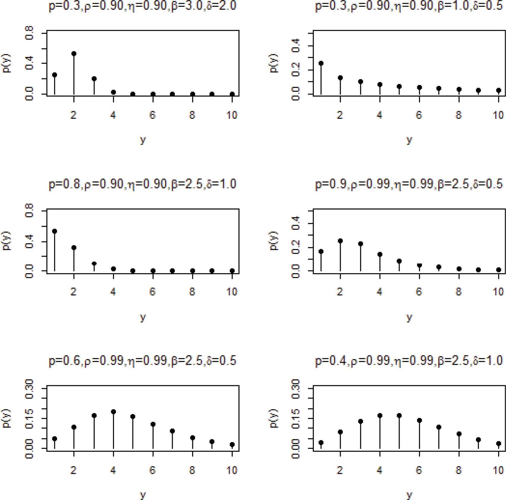
Figure 1, provides pmf plots of DAWGp,ρ,η,β,δ distribution for various choices of parameter values. The probabilities can be calculated recursively using the following relation:

pYy+1=1−pρyβηyδρy+1βηy+1δ−ρy+2βηy+2δ1−pρy+2βηy+2δρyβηyδ−ρy+1βηy+1δpYy.

Figure 1

Plots of the probability mass function (pmf) of discrete additive Weibull geometric (DAWG) (p, ρ, η, β, δ) distribution.

From Gupta et al. [27], we have the distribution having pmf pYy is log-concave if and only if pYy+1pYyy≥0 is decreasing and log-convex if and only if pYy+1pYyy≥0 is increasing. Also, if the sequence pYy+1pYyy≥0 is constant, then the hazard rate is constant and the distribution is geometric.

The cdf of DAWGp,ρ,η,β,δ distribution is,

Fy;p,ρ,η,β,δ=PY≤y=1−SXy+PY=y=1−ρy+1βηy+1δ1−pρy+1βηy+1δ,
where y=0,1,2,…; β>δ>0 (or δ>β>0), 0<p<1,0<ρ<1 and 0<η<1. Here note that, F0=1−ρη1−pρη and the proportion of positive values is ρη1−p1−pρη.

The survival function of DAWGp,ρ,η,β,δ distribution is given by,

Sy=PY>y=1−PY≤y=1−pρy+1βηy+1δ1−pρy+1βηy+1δ.

The hazard rate function of DAWGp,ρ,η,β,δ distribution is

hy=PY=y/Y≥y=PY=yPY≥y=1−ρy+1β−yβηy+1δ−yδ1−pρy+1βηy+1δ,
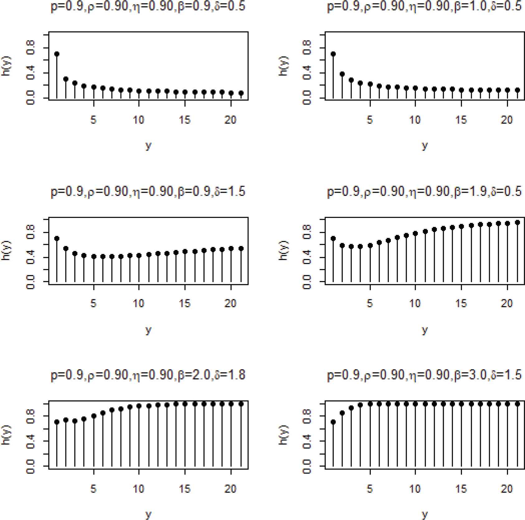
provided, PY≥y>0. In Figure 2, we present the plot of hazard rate function of DAWGp,ρ,η,β,δ distribution for various parameter values. When y→0, we have from Eq. (14)

Figure 2

Plots of the hazard rate function of discrete additive Weibull geometric (DAWG) (p, ρ, η, β, δ) distribution.

hy→1−ρη1−pρη=pY0.

Now to study the limit of hy as y→∞, we consider the following five cases based on the values of the shape parameters β and δ:

Case (i). When β>1 and δ>1 (provided β>δ or β<δ).

Here note that limy→∞hy=1. In this case h0=1−ρη1−pρη, h1=1−ρ2β−1η2δ−11−pρ2βη2δ, h2=1−ρ3β−2βη3δ−2δ1−pρ3βη3δ, … . That is, h0<h1<h2<…<1. Therefore, hy is an increasing function increases from 1−ρη1−pρη to 1.

Case (ii). When β>1 and δ=1.

Here note that limy→∞hy=1. Also it can be seen that h0<h1<h2<…<1. Therefore, hy is an increasing function increases from 1−ρη1−pρη to 1.

Case (iii). When 0<β<1 and δ>1.

Here also limy→∞hy=1. But here hy is initially decreases from h0 to the minimum point hm and then increases to 1. The minimum point m can be numerically identified by solving the conditions, hm−hm−1≤0 and hm+1−hm≥0.

Case (iv). When 0<β<1 and δ=1.

In this case limy→∞hy=1−η. Also h0>h1>h2>…>1−η. That is, hy is a decreasing function.

Case (v). When 0<β<1 and 0<δ<1 (provided β>δ or β<δ).

Here limy→∞hy=0. It can be shown that h0>h1>h2>…>0. That is, in this case also, hy is decreasing.

Figure 3, shows a comparison of all the five cases explained above.
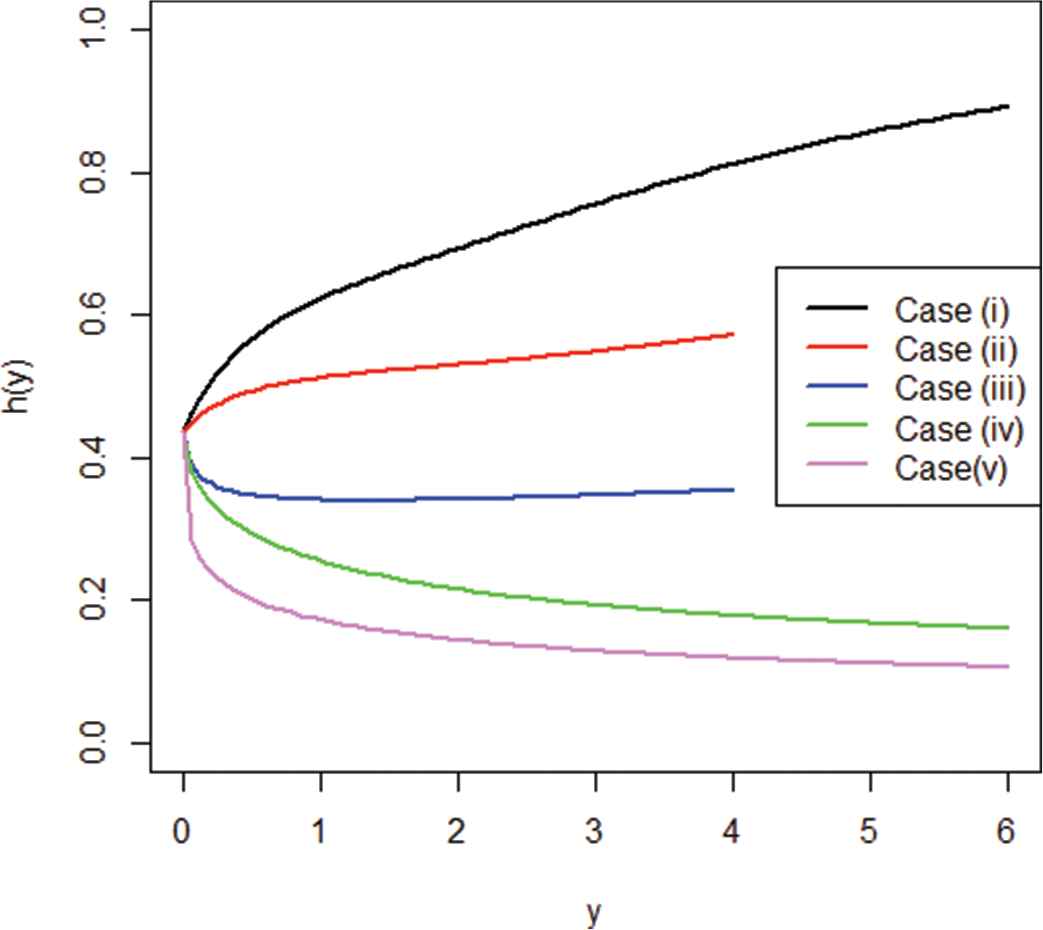
Figure 3

Plots of the hazard rate functions for the five cases.

The reverse hazard rate function is

h*y=PY=y/Y≤y=1−pρyβηδ−ρy+1βηy+1δ1−pρyβηδ1−ρy+1βηy+1δ.

The second rate of failure is

h**y=logSySy+1=log1ρy+2β1ηy+2δ−p1ρy+1β1ηy+1δ−p.

The accumulated hazard function, Hy is given by,

Hy=∑t=0yht=∑t=0y1−ρt+1β−tβηt+1δ−tδ1−pρt+1βηt+1δ.

The mean residual life function (MRLF) is given by,

Ly=EY−y|Y≥y=∑j>ySjSy=∑j≥y∏t=yj1−hi=∑j≥y∏i=yjρi+1βηi+1δ1−pρiβηiδρiβηiδ1−pρi+1βηi+1δ; y=0,1,2, … .

3.1. Quantile Function

Since the cdf of DAWG distribution is not invertible, we use the method discussed in Lemonte et al. [25] to obtain the quantile function. We take

Fy=1−ρy+1βηy+1δ1−pρy+1βηy+1δ=u,
where u∈0,1. This implies,
y+1βlnρ+y+1δlnη=ln1−u1−up.

We obtain the nonlinear equation, atβ+ctδ=x, where a=lnρ,c=lnη,x=ln1−u1−up and t=y+1. We can expand tβ in Taylor series as tβ=∑k=0∞βkt−1k/k!=∑k=0∞fjtj, where fj=∑k=j∞−1k−jkjβk/k!, βk=ββ−1…β−k+1 is the falling factorial and βk=ββ+1…β+k−1 is the ascending factorial. Analogously, we can expand tδ as tδ=∑j=0∞gjtj, where gj=∑k=j∞−1k−jkjδk/k!. Now,

x=Ht=∑j=0∞afj+cgjtj=∑j=0∞hjtj,
where hj=afj+cgj. To obtain an expansion for the quantile function of DAWG distribution we use the Lagrange's theorem. Now suppose that if the power series expansion holds
x=Ht=h0+∑j=1∞hjtj, h1=H′t|t=0≠0,
where Ht is analytic at a zero point, then the inverse power series t=H−1x exists and is single-valued in the neighbourhood of the point x=0, and is given by
t=H−1x=∑j=1∞υjxj,
where the coefficients υj are given by
υj=1j!dj−1dtj−1ϕtj|t=0, ϕt=tHt−h0.

Hence, the quantile function can be expressed as

Qu=∑j=1∞υjln1−u1−upj−1.

3.2. Moments

The rth raw moment about origin is given by,

μr′=EYr=∑y=0∞yr1−pρyβηyδ−ρy+1βηy+1δ1−pρyβηyδ1−pρy+1βηy+1δ.

Since this expansion is not in a tractable form, for given values of p,ρ,η,β and δ, the moments can be numerically computed using R programming. Table 1 shows the moments, skewness and kurtosis for DAWG distribution for given values of parameters.

Parameter Raw moments Central moments Skewness Kurtosis
μ1′=0.27
β=1.5 μ2′=0.45  μ2=0.38
δ=2 μ3′=0.98  μ3=0.65 2.79 12.59
μ4′=2.70  μ4=1.82
μ1′=0.32
β=1.5 μ2′=0.73  μ2=0.63
δ=1 μ3′=2.37 u3=1.73 3.50 19.44
μ4′=10.24  μ4=7.59
μ1′=0.46
β=0.5 μ2′=1.76 μ2=1.55
δ=1.5 μ3′=10.13 μ3=7.88 4.09 25.18
μ4′=76.97 μ4=60.28
μ1′=1.38
β=0.2 μ2′=27.89 μ2=26.00
δ=0.9 μ3′=1092.96 μ3=983.02 7.41 86.06
μ4′=63894.82 μ4=58185.39
Table 1

Moments, skewness, and kurtosis for p=0.9, ρ=0.8, η=0.9, and various choices of β and δ.

3.3. Order Statistics

Let Y1,Y2,…,Yn be a random sample from DAWGp,ρ,η,β,δ distribution. Also, let Y1,Y2,…,Yn, denotes the corresponding order statistics. Then the pmf and the cdf of kth order statistic, say, Z=Yk, are

fZz=n!k−1!n−k!Fk−1z1−Fzn−kfz=n!k−1!n−k!1−pn−k+1ρn−kz+1βηn−kz+1δ1−pρz+1βηz+1δnρzβηzδ−ρz+1βηz+1δ1−ρz+1βηz+1δk−11−pρzβηzδ,
and
FZz=∑i=knnjFjz1−Fzn−j=∑j=knnj1−pn−jρn−jz+1βηn−jz+1δ1−ρ(z+1)βηz+1δj1−pρz+1βηz+1δn,
respectively.

The pmf of the minimum is,

fY1z=n1−pnρn−1z+1βηn−1z+1δρzβηzδ−ρz+1βηz+1δ1−pρzβηzδ1−pρz+1βηz+1δn,
and the pmf of the maximum is,
fYnz=n1−p1−ρz+1βηz+1δn−1ρzβηzδ−ρz+1βηz+1δ1−pρzβηzδ1−pρz+1βηz+1δn.

3.4. Stress–Strength Parameter

The stress-strength parameter, R=PY>Z is a measure of component reliability. Suppose that, the random variable Y is the strength of a component which is subjected to a random stress Z, the estimation of R when Y and Z are i.i.d has been considered in the literature. One may see Kotz et al. [28], for a review of stress-strength model. In the discrete case, the stress-strength model is defined as,

R=PY>Z=∑y=0∞pYyFZy,
where, pYy and FZy denotes the pmf and cdf of the independent discrete random variables Y and Z, respectively. The stress-strength models are applied in various fields such as Engineering, Psychology and Medicine.

Let, Y∼DAWGθ1 and Z∼DAWGθ2, where, θ1=p1,ρ1,η1,β1,δ1T and θ2=(p2, ρ2, η2, β2, δ2)T. Then, from Eq. (10) and Eq. (12), we have,

R=∑y=0∞1−p1ρ1yβ1η1yδ1−ρ1y+1β1η1y+1δ11−ρ2y+1β2η2y+1δ21−p1ρ1yβ1η1yδ11−p1ρ1y+1ta1η1y+1δ11−p2ρ2y+1β2η2y+1δ2.

Assume that, y1,y2,…,yn and z1,z2,…,zm are independent observations drawn from DAWGθ1 and DAWGθ2, respectively. The total likelihood function is given by, LRθ*=Lnθ1 Lmθ2, where, θ*=θ1, θ2. The score vector is given by,

URθ*=∂LR∂p1,∂LR∂ρ1,∂LR∂η1,∂LR∂β1,∂LR∂δ1,∂LR∂p2,∂LR∂ρ2,∂LR∂η2,∂LR∂β2,∂LR∂δ2.

The MLE, θ^* may be obtained from the solution of the nonlinear equation, URθ^*=0. Applying θ^*, in Eq. (26), the stress-strength parameter R can be obtained. The stress strength reliability function for different values of p1, ρ1, η1, β1, δ1 and p2, ρ2, η2, β2, δ2 are computed in Table 2. We see that the value of R is decreasing when β1 and δ1 increases, and increasing when β2 and δ2 increases.

p1=0.8,p2=0.8
ρ1=0.5,ρ2=0.5 η1=0.5,η2=0.5
β1,δ1→

β2,δ2↓
(0.5,1) (1,1.5) (1.5,2) (2,2.5)
0.5,1 0.9404 0.9402 0.9402 0.9401
1,1.5 0.9411 0.9410 0.9409 0.9409
1.5,2 0.9413 0.9413 0.9412 0.9412
(2,2.5) 0.9413 0.9413 0.9413 0.9413
ρ1=0.2,ρ2=0.6 η1=0.2,η2=0.6
β1,δ1→

β2,δ2↓
(0.5,1) (1,1.5) (1.5,2) (2,2.5)
0.5,1 0.8994 0.8993 0.8993 0.8993
1,1.5 0.8996 0.8996 0.8995 0.8995
1.5,2 0.8997 0.8997 0.8997 0.8996
(2,2.5) 0.8977 0.8997 0.8997 0.8997
p1=0.5,p2=0.8
ρ1=0.5,ρ2=0.5 η1=0.5,η2=0.5
β1,δ1→

β2,δ2↓
(0.5,1) (1,1.5) (1.5,2) (2,2.5)
0.5,1 0.9443 0.9438 0.9436 0.9435
1,1.5 0.9457 0.9455 0.9454 0.9453
1.5,2 0.9463 0.9462 0.9462 0.9461
(2,2.5) 0.9464 0.9464 0.9464 0.9463
ρ1=0.2,ρ2=0.6 η1=0.2,η2=0.6
β1,δ1→

β2,δ2↓
(0.5,1) (1,1.5) (1.5,2) (2,2.5)
0.5,1 0.9002 0.9001 0.9001 0.9001
1,1.5 0.9006 0.9006 0.9005 0.9005
1.5,2 0.9008 0.9008 0.9008 0.9008
(2,2.5) 0.9009 0.9009 0.9009 0.9009
Table 2

Value of R for various choices of parameter values.

4. MAXIMUM LIKELIHOOD ESTIMATION (MLE) OF PARAMETERS

Consider a random sample y1,y2,…,yn of size n from the DAWGp,ρ,η,β,δ distribution. Then, the likelihood function is given by,

L=1−pn∏i=1nρyiβηyiδ−ρyi+1βηyi+1δ∏i=1n1−pρyiβηyiδ∏i=1n1−pρyi+1βηyi+1δ.

The log-likelihood function is,

logL=nlog1−p+∑i=1nlogρyiβηyiδ−ρyi+1βηyi+1δ−∑i=1nlog1−pρyiβηyiδ−∑i=1nlog1−pρyi+1βηyi+1δ.

The likelihood equations are the following:

∂logL∂p=−n1−p+∑i=1nρyiβηyiδ1−pρyiβηyiδ+∑i=1nρyi+1βηyi+1δ1−pρyi+1βηyi+1δ=0,
∂logL∂ρ=∑i=1nyiβρyiβ−1ηyiδ−yi+1βρyi+1β−1ηyi+1δρyiβηyiδ−ρyi+1βtayi+1δ+ p∑i=1nyiβρyiβ−1ηyiδ1−pρyiβηyiδ+p∑i=1nyi+1βρyi+1β−1ηyi+1δ1−pρyi+1βηyi+1δ=0,
∂logL∂η=∑i=1nyiδρyiβηyiδ−1−yi+1δρyi+1βηyi+1δ−1ρyiβηyiδ−ρyi+1βηyi+1δ+ p∑i=1nyiδρyiβηyiδ−11−pρyiβηyiδ+p∑i=1nyi+1δρyi+1βηyi+1δ−11−pρyi+1βηyi+1δ=0,
∂logL∂β=logρ∑i=1nyiβρyiβηyiδlogyi−yi+1βρyi+1βηyi+1δlogyi+1ρyiβηyiδ−ρyi+1βηyi+1δ+plogρ∑i=1nyiβρyiβηyiδlogyi1−pρyiβηyiδ+plogρ∑i=1nyi+1βρyi+1βηyi+1δlogyi+11−pρyi+1βηyi+1δ=0,
and
∂logL∂δ=logη∑i=1nyiδρyiβηyiδlogyi−yi+1δρyi+1βηyi+1δlogyi+1ρyiβηyil−ρyi+1βηyi+1δ+plogη∑i=1nyiβρyiβηyiδlogyi1−pρyiβηyiδ+plogη∑i=1nyi+1βρyi+1βηyi+1δlogyi+11−pρyi+1βηyi+1δ=0.

These equations do not have explicit solutions and they have to be obtained numerically by using the statistical softwares like nlm package in R programming.

We compute the maximized unrestricted and restricted log-likelihood ratio (LR) test statistic for testing on some DAWG sub models. We can use the LR test statistic to check whether DAWG distribution for a given data set is statistically superior to the sub models. Here, H0:θ=θ0 versus H1:θ≠θ0 can be performed using LR test. The LR test statistic is ω=2lθ^,y−lθ^0,y, where θ^ and θ^0 are the MLEs under H1 and H0, respectively. The test statistic ω is asymptotically (as n→∞) distributed as χk2, where k is the length of the parameter vector θ of interest. The LR test rejects H0 if ω>χk,α2, where χk,α2 denotes the upper 1001−α% quantile of the χk2 distribution.

4.1. Simulation Study

Here we study the performance of the MLEs of the model parameters of DAWG distribution using Monte Carlo simulation for various sample sizes and for selected parameter values. The algorithm for the simulation study are given below:

  • step 1: Input the number of replications (N);

  • step 2: Specify the sample size n and the values of the parameters p,ρ,η,β and δ;

  • step 3: Generate ui∼Uniform0,1, i=1,2,…,n.;

  • step 4: Obtain random observations from DAWG distribution by solving for real roots of the Eq. (19) and take the floor value;

  • step 5: Compute the MLEs of the five parameters;

  • step 6: Repeat steps 3 to 5, N times;

  • step 7: Compute the average bias, mean square error (MSE) and coverage probability (CP) for each parameter.

Here the expected value of the estimator is Eθ^=1N∑i=1Nθ^i, average bias =1N∑i=1Nθ^i−θ, MSEθ^=1N∑i=1Nθ^i−θ2 and the CP = probability of θi∈θ^i±1.96−∂2logL∂θi2.

We have taken the parameter values as p=0.8,ρ=0.5,η=0.5,β=0.5 and δ=1.5 and generated random samples of size n = 20, 60 and 100 respectively. The MLEs of p,ρ,η,β and δ are determined by maximizing the log-likelihood function in Eq. (28) using the nlm package of R software based on each generated samples. This simulation is repeated 500 times and the average estimates of bias, MSE and CP are computed and presented in Table 3. It can be seen that, as the sample size increases, the bias and MSE decreases. Also note that the CP values are quite closer to the 95% nominal level.

Sample size Actual value Estimates Average bias MSE CP
p=0.8 0.921 0.115 0.074 0.873
ρ=0.5 0.346 −0.164 0.086 0.926
20 η=0.5 0.723 0.213 0.017 0.932
β=0.5 0.661 0.165 0.038 0.896
δ=1.5 1.833 0.301 0.099 0.882
p=0.8 0.866 0.071 0.016 0.926
ρ=0.5 0.486 −0.013 0.018 0.936
60 η=0.5 0.610 0.102 0.008 0.943
β=0.5 0.612 0.110 0.012 0.912
δ=1.5 1.598 0.096 0.073 0.917
p=0.8 0.833 0.028 0.009 0.938
ρ=0.5 0.491 −0.003 0.007 0.942
100 η=0.5 0.552 0.057 0.005 0.949
β=0.5 0.587 0.083 0.006 0.929
δ=1.5 1.554 0.052 0.011 0.934

MSE, mean square error; CP, coverage probability.

Table 3

The average bias, MSE, and CP for given values of parameters.

5. APPLICATION

In this section, to show how the DAWGp,ρ,η,β,δ distribution works in practice, we use the data set representing remission times (in months) of 128 bladder cancer patients taken from Lee and Wang [29]. The data are: 0.080 0.200 0.400 0.500 0.510 0.810 0.900 1.050 1.190 1.260 1.350 1.400 1.460 1.760 2.020 2.020 2.070 2.090 2.230 2.260 2.460 2.540 2.620 2.640 2.690 2.690 2.750 2.830 2.870 3.020 3.250 3.310 3.360 3.360 3.480 3.520 3.570 3.640 3.700 3.820 3.880 4.180 4.230 4.260 4.330 4.340 4.400 4.500 4.510 4.870 4.980 5.060 5.090 5.170 5.320 5.320 5.340 5.410 5.410 5.490 5.620 5.710 5.850 6.250 6.540 6.760 6.930 6.940 6.970 7.090 7.260 7.280 7.320 7.390 7.590 7.620 7.630 7.660 7.870 7.930 8.260 8.370 8.530 8.650 8.660 9.020 9.220 9.470 9.740 10.06 10.34 10.66 10.75 11.25 11.64 11.79 11.98 12.02 12.03 12.07 12.63 13.11 13.29 13.80 14.24 14.76 14.77 14.83 15.96 16.62 17.12 17.14 17.36 18.10 19.13 20.28 21.73 22.69 23.63 25.74 25.82 26.31 32.15 34.26 36.66 43.01 46.12 79.05.

Since the data set is continuous, here first we discretize the data by considering the floor value (y). The parameters are estimated by using the method of MLE. We compare the fit of the DAWG distribution with the discrete life time distributions:

  1. Geometric (G) distribution having pmf,

    PY=y=1−ppy; 0<p<1,y=0,1,2,… .

  2. Discrete Weibull (DW) distribution having pmf,

    PY=y=qyβ−qy+1β; 0<q<1,β>0,y=0,1,2,… .

  3. Discrete Logistic (DLOG) distribution (see Chakraborty and Chakravarty [30]) having pmf,

    PY=y=1−ppy−μ1+py−μ1+py−μ+1; 0<p<1,−∞<μ<∞, y=0,±1,±2,… .

  4. Exponentiated discrete Weibull (EDW) distribution (see Nekoukhou and Bidram [31]) having pmf,

    PY=y=1−py+1αγ−1−pyαγ; 0<p<1,α>0,γ>0,y=0,1,2,… .

  5. DWG distribution (see Jayakumar and Babu [21]) having pmf,

    PY=y=1−pρyα−ρy+1α1−pρyα1−pρy+1α,

where y=0,1,2,…; α>0, 0<p<1 and 0<ρ<1.

The values of the log-likelihood function −logL, the statistics Kolmogorov–Smirnov (K−S), Akaike Information Criterion (AIC ), Akaike Information Criterion with correction (AICC), and Bayesian Information Criterion (BIC) are calculated for the six distributions in order to verify which distribution fits better to these data. The better distribution corresponds to smaller −logL, AIC, AICC, BIC, and K−S values and larger p value.

Here, AIC=−2logL+2k, AICC=−2logL+2knn−k−1 and BIC=−2logL+klogn, where L is the likelihood function evaluated at the maximum likelihood estimates, k is the number of parameters, and n is the sample size. The K−S distance, Dn=supy|Fy−Fny|, where, Fny is the empirical distribution function.

The values in Table 4, indicates that DAWG distribution leads to a better fit compared to the other five models. Figure 4 shows the structure of the cdf's of the six models with the empirical distribution of the given data. Here the dotted line indicates the empirical cdf of the data. The LR test statistic is used to test the hypothesis H0:η=1 versus H1:η≠1 is ω=8.094>5.991 with p value 0.0175. So we reject the null hypothesis.

Model ML estimates -log L AIC AICC BIC K-S p value
G p^=0.8991 414.836 831.672 831.704 831.779 0.1000 0.1549
DW q^=0.9114 414.556 833.112 837.304 833.326 0.1131 0.0758
β^=1.0511
DLOG p^=0.8000 456.825 917.650 917.746 917.864 0.1860 0.0003
μ^=7.6149
p^=0.4689 409.766 825.532 825.726 825.854 0.1237 0.0399
EDW α^=0.5397
γ^=4.9697
p^=0.9529 409.277 824.554 824.748 824.876 0.0905 0.2458
DWG ρ^=0.9982
α^=1.7025
p^=0.9589 405.230 820.460 820.952 820.996 0.0882 0.2727
ρ^=0.9989
DAWG η^=0.9995
β^=1.7018
δ^=1.7016

−logL, log-likelihood function; K−S, Kolmogorov–Smirnov; AIC, Akaike Information Criterion; AICC, Akaike Information Criterion with correction; BIC, Bayesian Information Criterion; DLOG, Discrete Logistic; DAWG, discrete additive Weibull geometric; EDW, exponentiated discrete Weibull; DWG, discrete Weibull geometric; DW, discrete Weibull.

Table 4

Parameter estimates and goodness of fit for various models fitted for the data set.
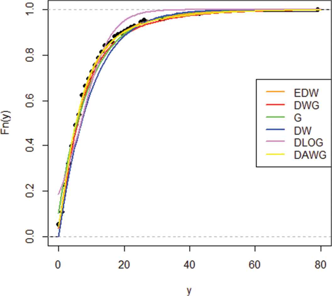
Figure 4

Fitted cumulative distribution function's (cdf) of the data with empirical distribution.

6. CONCLUSION

In the present study, we have introduced the generalized DAWG distribution. A particular member of this distribution, namely DAWG distribution is studied in detail. This discrete distribution contains the DWG, discrete exponential geometric, discrete modified Weibull, discrete Weibull, discrete Rayleigh, and geometric distribution as special cases. We have studied some basic properties of the new model and illustrated that the hazard rate function of the new model is monotonically increasing, decreasing, or bathtub shape depending on the values of the shape parameters. By fitting the DAWG model to a real data set, the flexibility and capacity of the new distribution in data modeling is established.

ACKNOWLEDGMENTS

The authors would like acknowledge the comments and suggestions of the Editor and the anonymous referee on earlier version of the manuscript which resulted in substantial improvements in the original version and presentation of the article.

REFERENCES

17.S. Chakraborty and D. Chakravarty, 2014. arXiv: 1410.7568[math.ST]
20.S. Chakraborty and D. Bhati, SORT, Vol. 40, 2016, pp. 153-176.
31.V. Nekoukhou and H. Bidram, SORT, Vol. 39, 2015, pp. 127-146.
Journal
Journal of Statistical Theory and Applications
Volume-Issue
18 - 1
Pages
33 - 45
Publication Date
2019/04/22
ISSN (Online)
2214-1766
ISSN (Print)
1538-7887
DOI
10.2991/jsta.d.190306.005How to use a DOI?
Copyright
© 2019 The Authors. Published by Atlantis Press SARL.
Open Access
This is an open access article distributed under the CC BY-NC 4.0 license (http://creativecommons.org/licenses/by-nc/4.0/).

Cite this article

TY  - JOUR
AU  - K. Jayakumar
AU  - M. Girish Babu
PY  - 2019
DA  - 2019/04/22
TI  - Discrete Additive Weibull Geometric Distribution
JO  - Journal of Statistical Theory and Applications
SP  - 33
EP  - 45
VL  - 18
IS  - 1
SN  - 2214-1766
UR  - https://doi.org/10.2991/jsta.d.190306.005
DO  - 10.2991/jsta.d.190306.005
ID  - Jayakumar2019
ER  -