
Bayes and Non-Bayes Estimation of Change Point in Nonstandard Mixture Inverse Weibull Distribution
Corresponding author. Email: mganji@uma.ac.ir
- DOI
- 10.2991/jsta.d.190306.011How to use a DOI?
- Keywords
- Bayes estimate; change point; mixture distribution; inverse Weibull distribution; maximum likelihood estimate
- Abstract
We consider a sequence of independent random variables
- Copyright
- © 2019 The Authors. Published by Atlantis Press SARL.
- Open Access
- This is an open access article distributed under the CC BY-NC 4.0 license (http://creativecommons.org/licenses/by-nc/4.0/).
1. INTRODUCTION
It is generally recognized that a physical entity experiences a structural change as it evolves over time. Such structural change problem are often used to describe abrupt changes in the mechanism underlying a sequence of random measurements. Further, in many real-life problems theoretical or empirical deliberations suggest models with occasionally changing one or more of its parameters. There is enormous frequentist and Bayesian literature on problems of detecting the change, inference concerning the change point, and related problems for various statistical models.
Control charts are one of the most important tools in statistical process control to monitor manufacturing processes and services. When a control chart shows an out-of-control condition, a search begins to identify and eliminate the root cause(s) of the process disturbance. The time when the disturbance has manifested itself to the process is referred to as change point. Identification of the change point is considered as an essential step in analyzing and eliminating the disturbance source(s) effectively.
Nonstandard mixture inverse Weibull (IW) distribution happens in many applied situations, for instance; life of a unit may have a IW distribution but some of the units fail instantaneously. In the study of tooth decay, the number of surfaces in a mouth which are filled, missing, or decayed are scored to produce a decay index. Healthy teeth are scored (0) for no evidence of decay. The distribution is a mixture of a mass point at (0) and a nontrivial continuous distribution of decay score. In the study of tumor characteristics, two variates can be recorded. A discrete variable to indicate the absence (0) or presence (1) of a tumor and a continuous variable measuring the tumor size.
A sequence of random variables
2. CHANGE POINT MODEL
Let the sequence of observations
3. BAYES ESTIMATORS OF PARAMETERS
The likelihood function of the given sample information is
Let
For Bayesian estimation, we need to specify a prior distribution for the parameters. As in Broemeling and Tsurumi [9], suppose that the marginal prior distribution for m is discrete uniform over the set
As in Calabria and Pulcini [10] and Erto and Guida [11], we assume that some prior information on the mechanism of failures in terms of reliability level at a prefixed time value are available. In addition, we assume that these prior technical information are given in terms of mean values
If the prior information is given in terms of the prior means
Making change of variables
Suppose the marginal prior distributions of
Mean and standard deviation of
For
Then, the joint prior distribution of
Also, the joint posterior distribution of
So, the marginal posterior distribution of
3.1. Point Estimation under Symmetric Loss Functions
In Bayesian framework a loss function is used to minimize the expected loss an estimator generates. The Bayes estimator of a generic parameter (or function thereof)
The Bayes estimators of
Other Bayes estimators of change point under loss functions,
3.2. Point Estimation under Asymmetric Loss Functions
In this section, we obtain Bayes estimator of change point under Linex loss function. The Linex loss function, proposed by Varian (1975) and discussed its behavior by Zellner (1986), is defined as
Calabria and Pulcini [13] introduced the following asymmetric loss function
This loss function is known as general entropy loss function (GEL). The Bayes estimate of change point, m, under GEL is
Also, the Bayes estimates of
4. MAXIMUM LIKELIHOOD ESTIMATORS
In this section, we obtain the maximum likelihood estimate of change point. We suppose
Then, the maximum likelihood estimates of
So, the maximum likelihood estimate of change point is the value of m which maximize the likelihood function
5. NUMERICAL STUDY, SENSITIVITY ANALYSIS OF BAYES ESTIMATES
The data given in Table 1 is a random sample of size n = 20 which is generated by using R-programming from the introduced change point model. We considered m = 10, its mean that, the change point in sequence is occurred after
| 1 | 2 | 3 | 4 | 5 | 6 | 7 | 8 | 9 | 10 | |
|---|---|---|---|---|---|---|---|---|---|---|
| 2.72 | 4.40 | 11.94 | 6.91 | 25.15 | 4.53 | 261.35 | 0 | 46.18 | 0 | |
| 11 | 12 | 13 | 14 | 15 | 16 | 17 | 18 | 19 | 20 | |
| 0 | 0.10 | 0.12 | 0.07 | 0.16 | 0.06 | 0 | 0 | 0.17 | 0 |
IW, inverse Weibull.
Generated observations from mixture of IW and degenerate distribution.
| Bayes estimates of change point | |||
|---|---|---|---|
| Prior | Posterior median | Posterior mode | |
| Informative | 10 | 10 | 10 |
The values of Bayes estimators of change point.
| Bayes estimates of proportions | ||
|---|---|---|
| Prior | Posterior mean | Posterior mean |
| Informative | 0.83 | 0.62 |
The values of Bayes estimators of proportions
| Prior | Bayes estimates of proportions | ||
|---|---|---|---|
| Informative | −2 | 0.84 | 0.63 |
| −1 | 0.83 | 0.62 | |
| 0.09 | 0.82 | 0.60 | |
| 0.5 | 0.81 | 0.59 | |
| 0.9 | 0.84 | 0.58 | |
The Bayes estimates using general entropy loss.
The results of Bayes estimates of change point, m, under Linex Loss function and GEL function by considering the different values of the shape parameters
| Prior | Shape parameter | Bayes estimates of change point | ||
|---|---|---|---|---|
| Iinformative | 2 | −2 | 11 | 10 |
| −1 | −1 | 10 | 10 | |
| 0.09 | 0.09 | 9 | 10 | |
| 0.5 | 0.5 | 9 | 9 | |
| 0.9 | 0.9 | 8 | 9 | |
The Bayes estimates using asymmetric loss functions.
| 0.95 | 0.05 | 10 |
| 0.85 | 0.05 | 9 |
| 0.75 | 0.05 | 9 |
| 0.95 | 0.04 | 10 |
| 0.95 | 0.03 | 10 |
| 0.95 | 0.02 | 9 |
| 0.85 | 0.01 | 9 |
| 0.75 | 0.01 | 9 |
SEL, symmetric loss function.
The Bayes estimates of m under SEL function for different values of μ1 and μ2.
| 0.8 | 0.6 | 10 |
| 0.7 | 0.6 | 10 |
| 0.6 | 0.6 | 10 |
| 0.8 | 0.5 | 10 |
| 0.8 | 0.4 | 10 |
| 0.8 | 0.3 | 10 |
| 0.7 | 0.5 | 10 |
SEL, symmetric loss function.
The Bayes estimates of m under SEL function for different values of μ3 and μ4.
| 0.8 | 0.6 | 0.83 | 0.62 | 0.81 | 0.59 | 0.84 | 0.63 |
| 0.8 | 0.5 | 0.84 | 0.59 | 0.85 | 0.57 | 0.84 | 0.61 |
| 0.7 | 0.6 | 0.80 | 0.60 | 0.79 | 0.59 | 0.82 | 0.63 |
| 0.7 | 0.5 | 0.80 | 0.60 | 0.79 | 0.56 | 0.82 | 0.61 |
| 0.6 | 0.6 | 0.78 | 0.61 | 0.76 | 0.60 | 0.79 | 0.63 |
| 0.6 | 0.5 | 0.77 | 0.60 | 0.77 | 0.56 | 0.79 | 0.62 |
Bayes estimates of proportions.
| 1 | 1 | 0.15 | 2 | 2.3 |
| 2 | 2 | 0.17 | 2 | 0.90 |
| 3 | 3 | 0.20 | 3 | 0.5 |
| 4 | 4 | 0.25 | 4 | 0.30 |
| 5 | 5 | 0.26 | 5 | 0.25 |
| 6 | 6 | 0.29 | 6 | 0.24 |
| 7 | 7 | 0.31 | 7 | 0.27 |
| 8 | 8 | 0.35 | 8 | 0.22 |
| 9 | 9 | 0.37 | 9 | 0.21 |
| 10 | 10 | 0.38 | 10 | 0.16 |
| 11 | 11 | 0.39 | 11 | 0.15 |
| 12 | 12 | 0.40 | 12 | 0.18 |
| 13 | 13 | 0.40 | 13 | 0.23 |
| 14 | 14 | 0.42 | 14 | 0.24 |
| 15 | 15 | 0.45 | 15 | 0.22 |
| 16 | 16 | 0.48 | 16 | 0.30 |
| 17 | 17 | 0.48 | 17 | 0.33 |
| 18 | 18 | 0.35 | 18 | 0.34 |
| 19 | 19 | 0.10 | 18 | 2.9 |
MSE, mean square error.
The values of MSE estimates of change point.
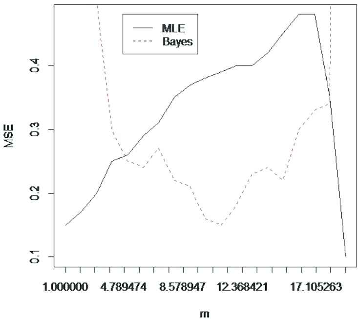
Comparison of Bayes and MLE estimators.
We would like to thank the referees for a careful reading of our paper and lot of valuable suggestions on the first draft of the manuscript.
REFERENCES
Cite this article
TY  - JOUR
AU  - Masoud Ganji
AU  - Roghayeh Mostafayi
PY  - 2019
DA  - 2019/03/31
TI  - Bayes and Non-Bayes Estimation of Change Point in Nonstandard Mixture Inverse Weibull Distribution
JO  - Journal of Statistical Theory and Applications
SP  - 79
EP  - 86
VL  - 18
IS  - 1
SN  - 2214-1766
UR  - https://doi.org/10.2991/jsta.d.190306.011
DO  - 10.2991/jsta.d.190306.011
ID  - Ganji2019
ER  -