We consider the purely sequential procedure for estimating the scale parameter of a gamma distribution with known shape parameter, when the risk function is bounded by the known preassigned number. In this paper, we provide asymptotic formulas for the expectation of the total sample size. Also, we propose how to adjust the stopping variable so that the risk is uniformly bounded by a known preassigned number. In the end, the performances of the proposed methodology are investigated with the help of simulations and also by using a real data set.
The problem of sequential estimation refers to any estimation technique for which the total number of observations used is not a degenerate random variable. In some statistical problems, especially in estimation fields, the sequential estimation must be used because no procedure based on fixed sample size can achieve the desired objective. Working with a sequential sampling procedure is necessary for some estimation problems with unknown parameters.
Sequential estimation of the scale parameter of a gamma distribution was first considered by Woodroofe [1], but this problem has not attracted attention from authors. Only Takada and Nagata [2] and Zacks and Khan [3] studied the confidence intervals of the mean and scale parameter of a gamma distribution. Also, Isogai and Uno [4] considered the sequential procedure for estimating the mean of a gamma distribution when the loss function is squared error plus linear cost.
Recently, Mahmoudi and Roughani [5] studied the two-stage sampling procedure for estimating the scale parameter of a gamma distribution with known shape parameter. They provided explicit formulas for the distribution and expected value of the stopping variable. Also, Roughani and Mahmoudi [6] continued and completed the study of the two-stage sampling procedure for estimating the scale parameter of a gamma distribution that have been proposed by Mahmoudi and Roughani [5]. They provided explicit formulas for the expected value and risk of the estimator of a gamma scale parameter, where the shape parameter is known. In spite of a little work has been done on gamma distribution, many investigators focused on exponential distribution. Starr and Woodroofe [7], Mukhopadhyay [8], Isogai and Uno [9], Mukhopadhyay [10], Mukhopadhyay and Datta [11], Uno et al. [12], Zacks and Mukhopadhyay [13,14], Mukhopadhyay and Pepe [15], Zacks [16], Mahmoudi and Lalehzari [17], Lalehzari et al. [18] and some others introduced many methods for sequential estimation of the scale parameter of an exponential distribution.
Survival and reliability analysis are two important scientific fields of study where the gamma distribution is most often used to model data. In survival analysis, variables such as lifespan of organisms as well as time till a treatment takes effect can be modelled with the gamma distribution. In reliability studies, lifespan of a system or systems components as well as chemical corrosion, e.g. can be modelled with the gamma distribution. The information gained by these two statistical models, is used to develop life insurance plans, pertinent drug information, warranty information, quality control information, etc. A parameter often studied in these fields is Mean Time to Failure (MTTF) that is very useful for systems used on a regular basis (see, e.g., Amero and Bayarri [19]; Choe and Shroff [20]).
The study about the scale parameter of a gamma distribution with known shape parameter is important because of (i) one can check the robustness of an exponential distribution when the shape parameter in gamma distribution is known. (ii) To avoid very long computational time in detecting multiple change points in a gamma-distributed sample, previous change point detection algorithms usually assume a known shape parameter α (Killick and Eckley [21]). (iii) When modelling failure times with a known number of failures and missing values are present, the time between one failure and the last record is gamma with known shape. This happens often when data are recorded periodically and not after each failure. MTTF is often estimated as an exponential random variable, however in many cases, MTTF is modeled with a gamma distribution when the shape is known and not equal to one. Dopke [22] and Coit and Jin [23] discussed the estimation of the MTTF as a gamma random variable. The example given by Coit and Jin is when the time between each failure is not recorded. If there are k failures in a span t, then the MTTF is gamma distributed with known shape k and unknown scale. (iv) There are particular instances where the shape parameter is either known or can be assumed as known. These situations occur with modelling times and normal distribution; there are modelling times when the shape parameter is assumed known just as there are instances in the normal distribution when variance is assumed known. This can happen for a number of reasons; either there is so much historical evidence that the shape is consistent, there exists some mathematical theory for the shapes value, or the actual shape is of little concern as long as it is within reason. For example, Mareuil et al. [24] in precipitation models, discussed the actual unimportant of knowing the exact shape. They stated that since the data is right skewed, it is important to model the data with a low shape value. In this dissertation, they simply modelled precipitation intensity with α=2. (v) One cannot reduce the case of Gammaα,1 to that of Gamma1,1 if α is arbitrary, if α=1/2 then one could base the procedure on sums of two independent random variables and reduce the case to that of exponential jumps. But, this is not efficient and can be done only if α=1/i, for i=1,2,⋯, (Zacks and Khan, [3], p. 298). For more explanation about this item, consider the arrival process where the random variable Si denotes the time until the ith outcome is occurred, Xi is the time between i−1 and ith outcome and Nt as the Poisson process with rate λ denotes the number of outcomes until time t. We know that Xi=Si−Si−1 has exponential distribution with mean β=1/λ, Si=∑j=1iXj∼Gamma(i,β), i∈N and Nt∼Poissonλt. The random variable Xi,i∈N, with Gamma1,β can be denoted as sum Xi=∑j=1iXij, where Xij's are independent random variables with Gamma1/i,β distribution.
In this paper, we consider the purely sequential procedure for estimating the scale parameter of a gamma distribution, with known shape parameter, when the risk function is bounded by the known preassigned number ω>0. Also, we provide asymptotic formulas for the expected value of the total sample size, i.e., EN. We propose how to adjust the stopping variable N, so that the risk is uniformly bounded by a known preassigned number ω>0. In the end, the performances of the proposed methodology are investigated with the help of simulations and by using a real data set.
The reminder of the paper is organized as follows:
In Section 2, we introduce the purely sequential procedure which is used in this paper. The expected value and bias of N and β^N are calculated in Section 3. To investigate the results of the previous sections, a simulation study is carried out in Section 4. In Section 5, the purely sequential procedure based on adjusted N, i.e., Nadj, is introduced and its bias and expectation is obtained. We compare the two-stage and purely sequential procedures in Section 6. To investigate the results of this sequential problem, we use one application of a real data set in Section 7. Finally, Section 8 concludes the paper and discusses the results.
2. PURELY SEQUENTIAL PROCEDURE
Consider we observe a sequence of independent and identically distributed random variables X1,X2,⋯ from a gamma distribution, with common probability density function
fx;α,β=1Γαβαxα−1e−xβIx>0,
where the scale parameter β>0 is unknown, but the shape parameter α>0 is known.
Having observed X1,X2,⋯,Xn, let β is estimated by β^n=∑Xinα=X¯nα and the loss function in estimating β by β^n is given by
Lβ^n,β=Aβ^n−β2,
where A is a positive known weight.
Our goal is to make the risk function associated with this loss function less than a preassigned number ω>0, i.e.,
AEβ^n−β2≤ω.
The risk is Rβ^n,β=EAβ^n−β2=Aβ2αn, and this will be at most ω if n≥Aβ2αω=n∗. n∗ may not be an integer. It is called the optimal fixed sample size and remains unknown since β is unknown. Takada [25] showed that no procedure based on fixed sample size can solve this problem.
In the purely sequential procedure, n∗ is estimated successively in a sequential manner. One may begin with m≥2 observations and then continue to take one additional observation at a time, but terminate sampling when he has gathered enough observations. At each stage, he estimates β and translates it to estimate n∗, then checks whether the sample size exceeds the estimate of n∗. As soon as the sample size exceeds the estimate of n∗, the sampling is terminated and final estimate of β is offered.
The optimal sample size n∗=Aβ2αω is a function of unknown parameter β, hence we start with X1,X2,⋯,Xm, as pilot sample observations following the gamma distribution in (1). Then, we will proceed with one additional observation at a time, and terminate sampling according to the stopping time
N=infn≥m;n≥AX¯n2α3ω.
This procedure is worked as follows. In the initial stage, we compute X¯m based on X1,X2,⋯,Xm and check whether m≥AX¯m2α3ω. Note that AX¯m2α3ω is an estimatorof n∗ at this stage. If m≥AX¯m2α3ω, then we stop sampling and our final sample size is m, i.e., N=m. But, if m<AX¯m2α3ω we take one additional observation Xm+1 and update the sample mean by X¯m+1 based on X1,X2,⋯,Xm,Xm+1. Again, we check whether m+1≥AX¯m+12α3ω as an estimate of n∗ at this stage. If m+1≥AX¯m+12α3ω then sampling is terminated and N=m+1, else we must take another observation. This continues until we arrive at the sample size n for the first time which is at least as large as the associated estimator of n∗, namely AX¯n2α3ω. Hence, the final sample size is n, i.e, N=n. Finally, we use X1,X2,⋯,XN and introduce β^N=X¯Nα as a final estimator of β.
3. THE EXPECTED VALUE AND BIAS OF N AND β^N
If we consider (3), we find that the exact probability distribution of N is hard to compute. For example, let m=20 and the sequential sampling stopped with N=24. This means that we did not stop with 20, 21, 22 or 23 observations, but we stopped with 24 observations. In other words, the event N=24 is the same as the event
20<AX¯202α3ω,⋯,23<AX¯232α3ω and 24≥AX¯242α3ω,
and finding the probability of this event is very hard. But, we can compute the approximate expected value of N.
Let Gx,α,β denotes the cumulative distribution function (c.d.f.) of a gamma distribution with shape parameter α and scale parameter β, i.e., Gx,α,β=PX≤x where X∼Gammaα,β and G¯x,α,β=1−Gx,α,β.
Theorem 3.1.
(The first moment ofN) Suppose thatmα>2andr>2. Ifn∗>mthen
as ω→0. The bias is not always negative. Its negatively or positively depends on values of α. The values of
∑n=1∞G¯32nα,nα+1,1−32G¯32n,nα,1
is positive for each values of α and is decreasing as a function of α. Thus, the values of
−2∑n=1∞G¯32nα,nα+1,1−32G¯32nα,nα,1
is negative. Therefore, the bias of N, BiasN,n∗, may be negative or positive which depends on the values of α. For example for α=2, we have BiasN,n∗=−0.568 and for α=4, BiasN,n∗=0.0524.
Theorem 3.2.
The stopping timeNin(3), satisfies the second order asymptotic efficiency results, i.e., EN−n∗=O1.
Proof.
For proof this property, it is enough to show that ∑n=1∞G¯32nα,nα,1<∞ and ∑n=1∞G¯32nα,nα+1,1<∞.
For X∼Γnα+1,1 and t<1, using Chernoff inequality, we have
where MXt denotes the moment generating function of X and exists for t<1. Using first derivative test, it is easy to check that the function gt=e−32nαt1−t−nα−1 attains its global minimum at t=0.5nα−1/1.5nα which is less than 1 for all α. Hence,
Thus, ∑n=1∞G¯32nα,nα+1,1<∞, and hence, ∑n=1∞G¯32nα,nα,1≤∑n=1∞G¯32nα,nα+1,1<∞, since 1.5<e. The proof is completed.
Theorem 3.3.
Ifmα>2andr>2then the expectation ofβ^Nis
Eβ^N=β−2βαn∗+o1,
and its bias as a function ofβis given by
Biasβ^N,β=−2βαn∗+o1,
asω→0.
Proof.
The proof of this theorem is a special case of Theorem 5.2 for L0=0, presented in Section 5 of the paper.
We can use the result of this theorem and introduce a corrected estimator of β as follows:
β^Nc=X¯Nα+2X¯Nα2N=X¯Nα1+2αN.
This is an estimator with negligible bias and therefore, is better than β^N.
4. SIMULATION RESULTS
To investigate the results of the previous sections, a simulation study is carried out. We considered m=20, A=2, α=1 and 3.7 and β=1,2,⋯,25. For each set of values of A, m, α and β, we choose ω=2, 1, 0.5, 0.25, 0.1 and 0.05, so that n∗ was determined by Aβ2αω. Then, for any combination of m, α, β and ω, we ran h=10000 replications by letting R-program draws random samples from the assigned gamma population. Suppose that in the ith replication, we observe ni observations. Based on this data, the usual estimate of β is β^ni=x¯niα and its corrected estimate is β^nic=x¯niα1+2αni.
To summarize the results, we use the following notations:
E^N shows the simulated value of EN and is computed by n¯=h−1∑i=1hni.
E^β^N shows the simulated value of Eβ^N and is computed by h−1∑i=1hx¯niα.
The simulated bias of β^N is shown by B^β^N,β and its formula is E^β^N−β.
The simulated risk of β^N is shown by R^β^N,β and its formula is r¯=Ah−1∑i=1hx¯niα−β2.
E^β^Nc shows the simulated value of Eβ^Nc and is computed by h−1∑i=1hβ^nic.
The simulated bias of β^Nc is shown by B^β^Nc,β and its formula is E^β^Nc−β.
The simulated risk of β^Nc is shown by R^β^Nc,β and its formula is r¯c=Ah−1∑i=1hβ^nic−β2.
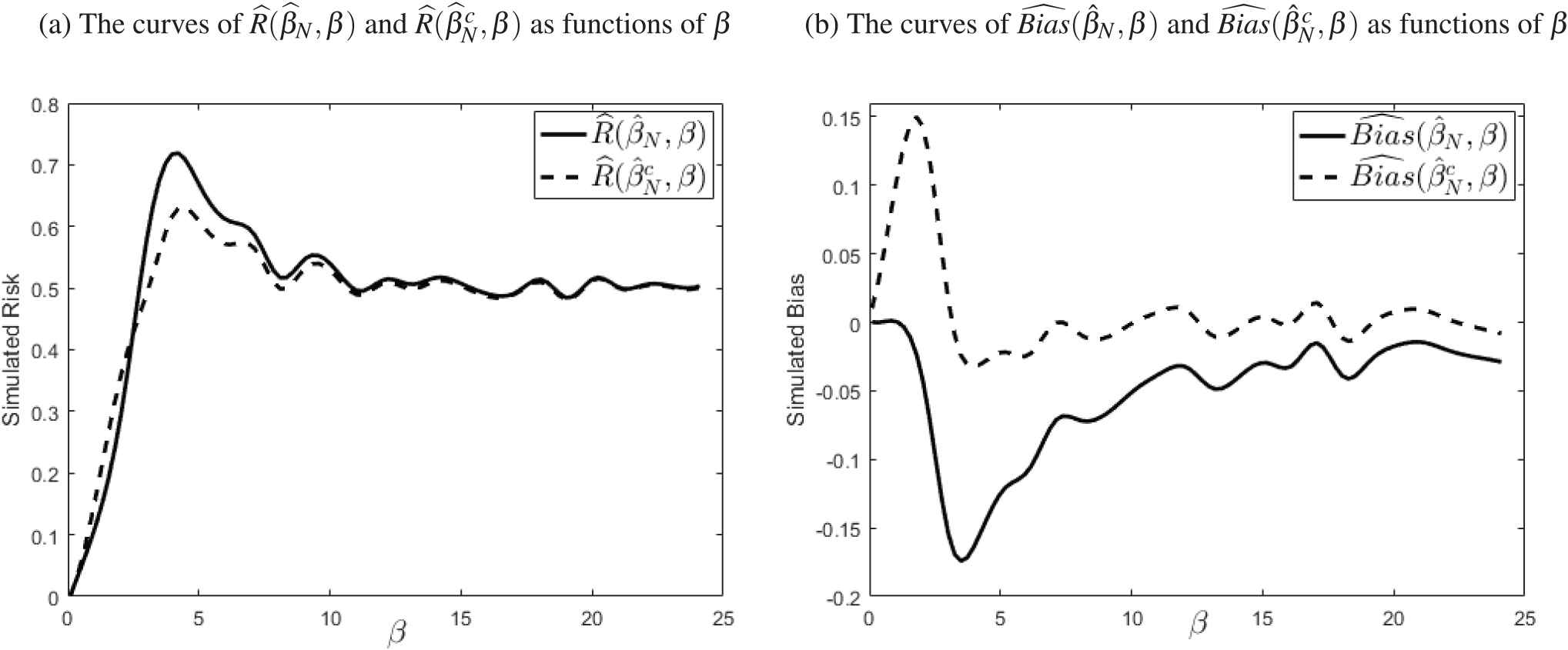
In Table 1, we present the results with β=5. Table 2 shows the results when ω expressed as a function of β. Fig. 1(a) compares R^β^N,β and R^β^Nc,β for different values of β. Also, Fig. 1(b) compares B^β^N,β and B^βNc,β for different values of β.
m=5, A=2, β=5, α=1
ω
2.000
1.000
0.500
0.250
0.100
0.050
n∗
25.000
50.000
100.000
200.000
500.000
1000.000
EN
23.068
48.068
98.068
198.068
498.068
998.068
E^N
21.872
45.896
96.401
197.400
497.440
998.222
Eβ^N
4.600
4.800
4.900
4.950
4.980
4.990
E^β^N
4.363
4.616
4.833
4.936
4.976
4.990
R^β^N,β/Rβ^n∗,β
2.160
2.522
2.016
1.427
1.202
0.993
E^β^Nc
4.822
4.841
4.939
4.987
4.996
5.000
R^β^Nc,β/Rβ^n∗,β
1.478
1.995
1.776
1.345
1.171
0.986
m=10, A=2, β=5, α=1
ω
2.000
1.000
0.500
0.250
0.100
0.050
n∗
25.000
50.000
100.000
200.000
500.000
1000.000
EN
23.068
48.068
98.068
198.068
498.068
998.068
E^N
23.392
47.109
97.356
197.681
497.828
997.396
Eβ^N
4.600
4.800
4.900
4.950
4.980
4.990
E^β^N
4.580
4.714
4.871
4.944
4.979
4.988
R^β^N,β/Rβ^n∗,β
1.358
1.763
1.466
1.137
1.055
1.007
E^β^Nc
5.003
4.929
4.974
4.994
4.999
4.998
R^β^Nc,β/Rβ^n∗,β
1.031
1.447
1.330
1.088
1.037
0.998
m=5, A=2, β=5, α=3.7
ω
2.000
1.000
0.500
0.250
0.100
0.010
n∗
6.757
13.514
27.027
54.054
135.135
270.270
EN
6.762
13.519
27.032
54.059
135.140
270.275
E^N
7.289
13.447
27.032
53.950
135.219
270.293
Eβ^N
4.600
4.800
4.900
4.950
4.980
4.990
E^β^N
4.757
4.778
4.895
4.944
4.981
4.990
R^β^N,β/Rβ^n∗,β
0.883
1.312
1.260
1.145
1.034
0.999
E^β^Nc
5.121
4.979
4.996
4.994
5.001
5.000
R^β^Nc,β/Rβ^n∗,β
0.795
1.120
1.163
1.097
1.019
0.991
Table 1
Simulations of purely sequential procedure under gamma distribution.
m=5, A=2, β=0.5, α=1
ω
0.1β
0.05β
0.025β
0.001β
n∗
10.000
20.000
40.000
1000.000
EN
8.068
18.068
38.068
998.068
E^N
9.652
17.604
36.142
998.592
Eβ^N
0.400
0.450
0.475
0.499
E^β^N
0.432
0.433
0.454
0.499
R^β^N,β/Rβ^n∗,β
1.022
1.821
2.424
0.998
E^β^Nc
0.528
0.489
0.482
0.500
R^β^Nc,β/Rβ^n∗,β
0.795
1.216
1.839
0.991
Table 2
Simulations of purely sequential procedure under gamma distribution when ω expressed as a function of β.
Figure 1.
The curves of simulated risk and bias as functions of β, for α=1,A=2,m=20 and ω=0.5.
Some of important observed features of simulation results are as follows:
As we expect, the exact and estimated values of EN are less than n∗.
The negativity of Bβ^N,β is verified.
The smaller value of ω, the better estimate of β.
The larger value of α, the better estimate of β and the smaller final sample size.
As we expect by Theorem 3.3, when the parameter β increases then B^β^N,β decreases.
When β is small, R^β^N,β, simulated risk, is less than ω, but this is not true at all and for some values β, we have R^β^N,β>ω.
When β is increasing to large values, the risk decreases and converges to ω.
As we expect, B^β^Nc,β is less than B^β^N,β and this verifies that, β^Nc is better than β^N as an estimator of β.
R^β^Nc,β is less than R^β^Nc,β, but still for some values β, the risk of β^Nc is greater than ω.
As we see, the two ratio R^β^N,β/R^β^n∗,β and R^β^Nc,β/R^β^n∗,β converge to 1 as w→0.
The second order asymptotic efficiency result, EN−n∗=O1, is seen in tables.
5. PURELY SEQUENTIAL PROCEDURE USING ADJUSTED N
Recall that we want to introduce an estimator of parameter β such that its associated risk is not greater than ω, but β^N and β^Nc did not have this property. Since the stopping time defined by (3) underestimates n∗, we believe that by adjusting N this problem can be solved.
To avoid underestimation at the termination, we consider the following stopping time
Nadj=infn≥m;Sn<α3ωAn1.5Ln,
where Ln=1+L0n+o1n as n→∞ and Ln>1 for any n. This stopping time is the adjusted version of (3), and is obtained by adding Ln to the right hand side of (3). Now, we can use (8) as a stopping time and run a purely sequential procedure. As soon as sampling terminate with this procedure, we define β^Nadj=X1+X2+⋯+XNadjαNadj=X¯Nadjα as an estimator of β. We will see that β^Nadj is a bias estimator of β.
Theorem 5.1.
(The first moment ofNadj) Suppose thatmα>2andr>2. Ifn∗>mthen
where Yi=Xiαβ and Zn=nLnY¯n2, the proof of this theorem is the same as proof of Theorem 2 of Takada and Nagata [2], thus we ignore to give the details.
By Theorem 5.2, we can correct the bias and introduce a corrected estimator as follows:
β^Nadjc=X¯Nadjα1+2αNadj.
The bias of this estimator is negligible and hence, is better than (12).
To find an appropriate Nadj, we have considered α=1, Ln=1+L0n+o1n and by empirical investigations saw that if we let L0=20 then we get the satisfactory results. Unfortunately, attempts to calculate the risk analytically has not let to a conclusion. Therefore, to resolve this captivity and to select a suitable value for L0, we use the simulation and empirical results with different values of the parameters involved in the model. The result of these extensive studies shows that the most appropriate value for L0 is 20.
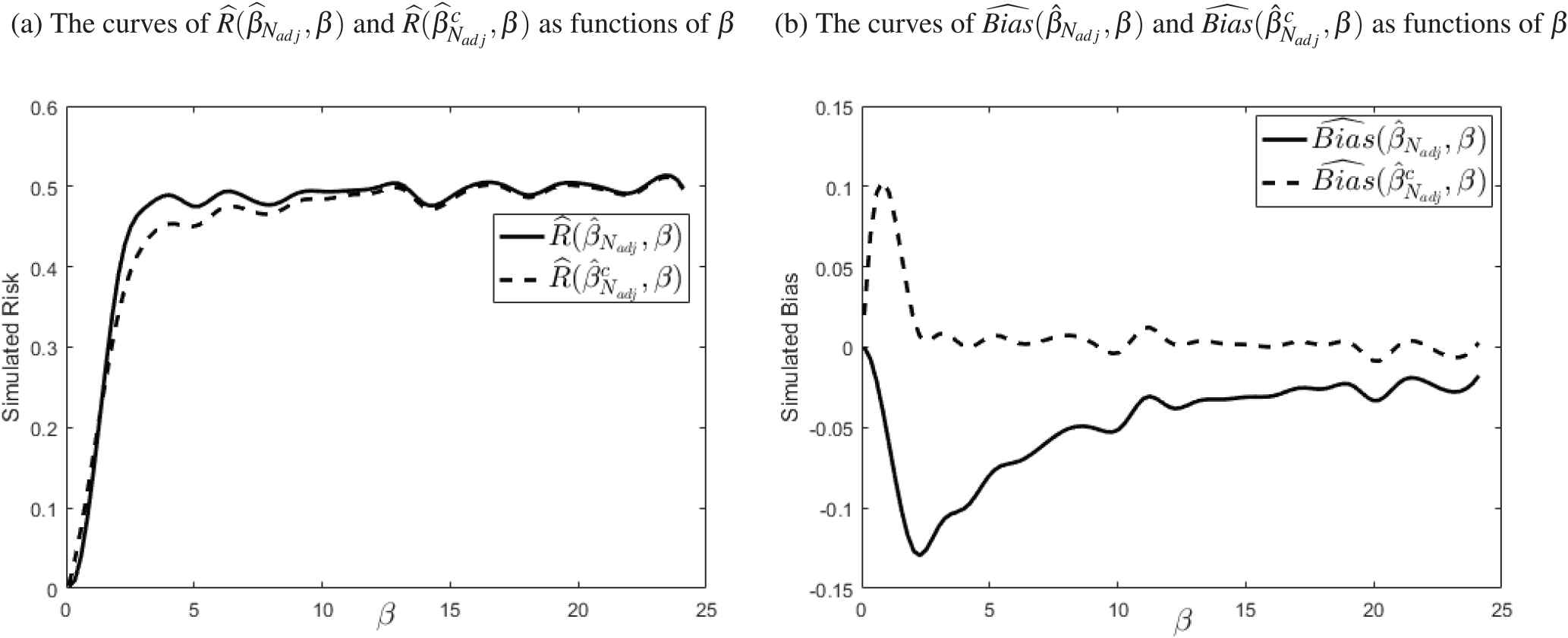
Table 3 shows the exact and simulated values of ENadj, Eβ^Nadj, R^β^Nadj,β, E^β^Nadjc and R^β^Nadjc,β. Table 4 shows the results with adjusted N when ω expressed as a function of β. Also, Fig. 2 shows the curves of simulated biases and simulated risks as functions of β. Since we want to compare the results of usual purely sequential procedure and purely sequential procedure with Nadj, all of the conditions in two simulations are the same except that here we use adjusted N as stopping time. Hence, one can compare Table 1 with Table 3, Table 2 with Table 4 and Fig. 1 with Fig. 2. This compare shows that when we use Nadj, the results improve. Also, the simulated results verify the superiority of β^Nadjc.
m=5, A=2, β=5, α=1
ω
2.000
1.000
0.500
0.250
0.100
0.050
n∗
25.000
50.000
100.000
200.000
500.000
1000.000
ENadj
43.068
68.068
118.068
218.068
518.068
1018.068
E^Nadj
36.996
63.841
115.344
216.719
517.556
1017.715
Eβ^Nadj
4.600
4.800
4.900
4.950
4.980
4.990
E^β^Nadj
4.754
4.844
4.911
4.955
4.981
4.990
R^β^Nadj,β/Rβ^n∗,β
0.977
1.004
0.986
1.007
0.986
0.984
E^β^Nadjc
5.017
4.999
4.997
5.001
5.001
5.000
R^β^Nadjc,β/Rβ^n∗,β
0.874
0.918
0.930
0.976
0.973
0.977
m=10, A=2, β=5, α=1
ω
2.000
1.000
0.500
0.250
0.100
0.050
n∗
25.000
50.000
100.000
200.000
500.000
1000.000
ENadj
43.068
68.068
118.068
218.068
518.068
1018.068
E^Nadj
36.793
63.994
115.624
216.735
517.910
1018.271
Eβ^Nadj
4.600
4.800
4.900
4.950
4.980
4.990
E^β^Nadj
4.741
4.853
4.918
4.956
4.983
4.992
R^β^Nadj,β/Rβ^n∗,β
0.894
0.963
0.960
0.992
0.977
0.977
E^β^Nadjc
5.004
5.008
5.004
5.002
5.003
5.001
R^β^Nadjc,β/Rβ^n∗,β
0.787
0.884
0.909
0.961
0.965
0.970
m=5, A=2, β=5, α=3.7
ω
2.000
1.000
0.500
0.250
0.100
0.050
n∗
6.757
13.514
27.027
54.054
135.135
270.270
ENadj
26.762
33.519
47.032
74.059
155.140
290.275
E^Nadj
15.765
24.804
40.619
69.855
152.920
289.025
Eβ^Nadj
4.600
4.800
4.900
4.950
4.980
4.990
E^β^Nadj
4.883
4.923
4.946
4.971
4.983
4.991
R^β^Nadj,β/Rβ^n∗,β
0.481
0.593
0.695
0.790
0.912
0.949
E^β^Nadjc
5.052
5.030
5.013
5.010
5.001
5.000
R^β^Nadjc,β/Rβ^n∗,β
0.463
0.574
0.676
0.777
0.901
0.942
Table 3
Simulations of purely sequential procedure with adjusted N under the gamma distribution.
m=5, A=2, β=0.5, α=1
ω
1β
0.05β
0.025β
0.001β
n∗
10.000
20.000
40.000
1000.000
ENadj
28.068
38.068
58.068
1018.068
E^Nadj
18.993
31.194
53.489
1018.625
Eβ^Nadj
0.400
0.450
0.475
0.499
E^β^Nadj
0.456
0.470
0.483
0.499
R^β^Nadj,β/Rβ^n∗,β
0.748
0.939
0.986
0.988
E^β^Nadjc
0.505
0.501
0.501
0.500
R^β^Nadjc,β/Rβ^n∗,β
0.641
0.827
0.901
0.982
Table 4
Simulations of purely sequential procedure with adjusted N under the gamma distribution when ω expressed as a function of β.
Figure 2
The curves of simulated risk and bias as functions of β for α=1,A=2,m=20 and ω=0.5 with adjusted N.
6. COMPARING PURELY SEQUENTIAL AND TWO-STAGE PROCEDURES
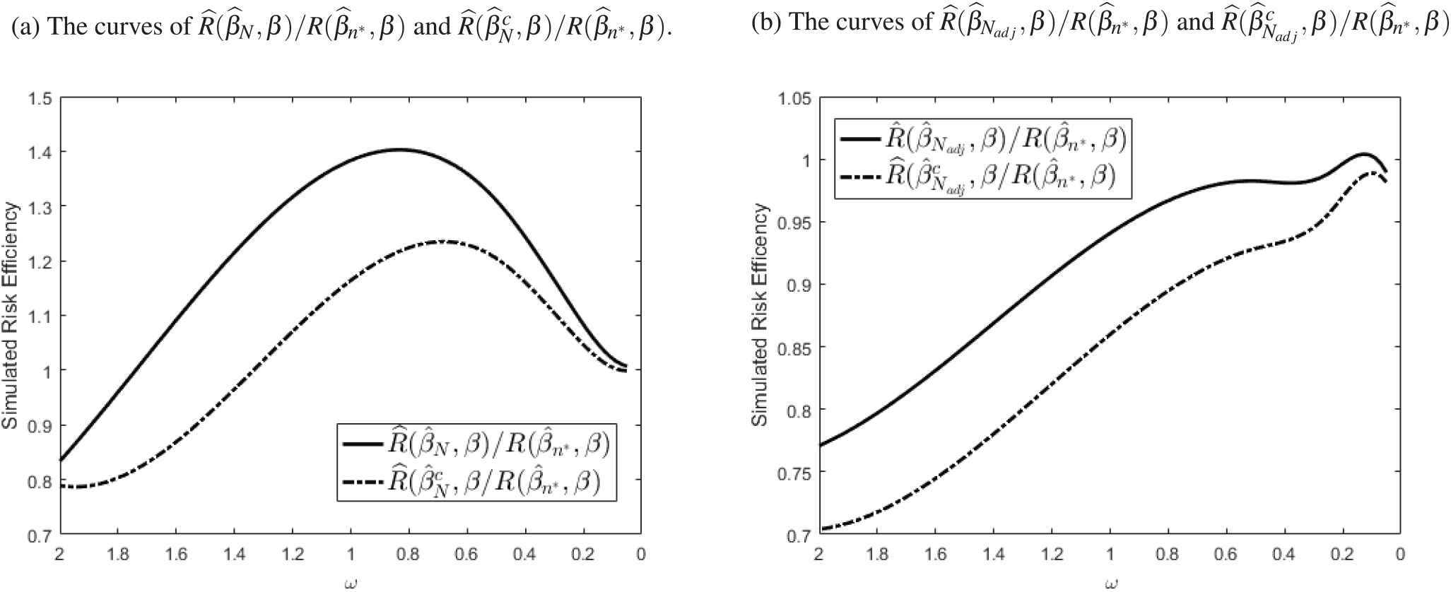
The two-stage procedure for estimating the scale parameter of a gamma distribution was introduced by Mahmoudi and Roughani [5]. The most important weakness of this procedure is oversampling. To reduce this weakness, the two-stage procedure was improved by Roughani and Mahmoudi [6], but the oversampling problem was not solved utterly. The purely sequential procedure reduces oversampling. Here, we compare the results of the improved two-stage procedure (two-stage procedure with Bnew) and the results of the purely sequential procedure. Table 5 shows the simulation results. The results show that for small values of ω, final sample size of purely sequential procedure is less than final sample size of two-stage procedure and this difference in size of samples is bolder for small values of α. In sequential estimation problem, we may expect risk efficiency to lie in a close proximity of one if ω tend to zero, so simulated risk efficiency is shown in Fig. 3.
m=20, A=2, β=5, α=1
ω
2.0000
1.0000
0.5000
0.2500
0.1000
0.0500
n∗
25.000
50.000
100.00
200.00
500.00
1000.0
Purely sequential
E^Nadj
37.470
63.829
115.85
216.76
517.66
1018.5
E^β^Nadj
4.8038
4.8465
4.9236
4.9555
4.9820
4.9921
R^β^Nadj,β
1.4925
0.9413
0.4784
0.2549
0.0982
0.0505
Two-stage
E^Nm
37.461
73.431
145.87
292.39
729.96
1457.8
E^β^Nm
4.7558
4.8372
4.9157
4.9568
4.9839
4.9916
R^β^Nm,β
1.5970
0.9782
0.4732
0.2240
0.0861
0.0427
m=20, A=2, β=5, α=3.7
ω
0.5000
0.2500
0.1000
0.0500
n∗
27.027
54.054
135.14
270.27
Purely sequential
E^Nadj
40.692
69.846
153.12
289.21
E^β^Nadj
4.9506
4.9700
4.9871
4.9925
R^β^Nadj,β
0.3544
0.1981
0.0913
0.0473
Two-stage
E^Nm
31.469
62.191
155.07
309.30
E^β^Nm
4.9177
4.9547
4.9815
4.9914
R^β^Nm,β
0.4778
0.2426
0.0937
0.0465
Table 5
Comparing the results of purely sequential and two-stage procedures.
Figure 3
Simulated risk efficiency as a function of ω for α=1,A=2,m=20.
7. REAL DATA
Zacks and Khan [3] provided a method to produce a random sample from gamma distribution using a random sample from normal distribution. This paper states that if Y1,⋯,Yn is a random sample from a normal distribution with mean μ and variance σ2, then the transformation i−1iYi−Y¯i−12, i>2 gives a random sample of size n−1 from gamma distribution with α=1/2 and β=2σ2.
In this section, we consider a dataset that consists of 346 observations of weights of babies born between September 2014, 23, and November 2014, 21, in Imam Ali hospital of Shahrekord in Iran. This dataset is given in Roughani and Mahmoudi [6]. This dataset is used to obtain real data from gamma population with known shape parameter α=1/2 and scale parameter β=2σ2. The mean and variance for the full data are 3.147 and 0.198 kg, respectively. The associated P-values according to goodness of fit test for normal and gamma distributions are 0.29 and 0.40, which made us feel reasonably assured of an underlying gamma distribution for transmuted dataset.
Treating transformed data set as the universe, we implemented purely sequential procedure, drawing observations from the full set of data as needed. Table 6 provides the results derived from implementing the stopping rules from (3), when the initial sample size m=5,10,20,25, ω=0.03 and A=2 are chosen arbitrarily. Under purely sequential procedure, the final estimators β^N tended to get closer to its true value β^=0.396 obtained from full data.
m=5
Pilot Data:
0.0658, 0.6411, 0.0903, 0.0162, 0.0316
β^m=0.338
Samples:
0.0515, 0.4734, 0.3122, 0.0681, 0.4683,
0.0652, 0.1088, 0.0001, 0.0932, 0.0361,
0.1117
→N=16β^N=0.3292
m=10
Pilot Data:
1.1970, 0.1248, 0.0003, 0.0658, 0.0349,
0.4524, 0.0001, 0.0149, 0.1679, 0.0785
β^m=0.4273
Samples:
0.0001, 0.2090, 0.3122, 0.1122, 0.0227,
0.0676, 0.1104
→N=17β^N=0.3495
m=20
Pilot Data:
0.5607, 0.0800, 0.2105, 0.0785, 0.0203,
0.7156, 0.1850, 0.0928, 0.5967, 0.0515,
0.5607, 0.1520, 0.1693, 0.0618, 0.0001,
0.1537, 0.2652, 0.1090, 0.0073, 0.1088
β^m=0.4180
Samples:
0.3907, 0.1679, 0.3907, 0.0020, 0.0336
→N=25β^N=0.4131
m=25
Pilot Data:
0.2044, 0.0958, 0.0361, 0.3223, 0.0001,
0.1112, 0.0553, 1.5112, 0.1653, 0.0289,
0.1245, 0.1445, 0.4910, 0.0534, 0.0252,
0.2466, 0.0252, 0.0443, 0.0275, 0.1319,
0.3227, 0.2161, 0.0581, 0.2518, 0.0580
Samples: initial samples is enough
→N=25β^N=0.3801
Table 6
An illustration of purely procedure with transformed data, when m=5,10,20,25, ω=0.03 and A=2.
8. CONCLUSION
Purely sequential sampling procedure is developed for estimating the scale parameter β in a gamma distribution with known shape parameter α. In this problem, the risk of an estimator β^ of β is less than from a preassigned number ω>0, i.e., Rβ^,β=AEββ^−β2≤ω, where 0<A<∞ is known. We compute asymptotic expressions for EN, Eβ^N and the bias of β^N. Also, we propose how to obtain the adjusted stopping variable Nadj so that the risk is uniformly bounded by a preassigned value ω. In the end, the performances of the proposed methodology are investigated with the help of simulations.
The problem of sequential estimation of scale parameter β where α is unknown is not easy to solve since the Maximum Likelihood Estimator (MLE) of α in a fixed sample size case, has not the explicit form. On the other hand, if one tries to use moment estimators of α and β, the problem is so hard because of the complexity of moments estimators of α and β. Recently, I and my colleagues start a work where the shape parameter α is not known, but very explicit formulas that obtain for known α can not be obtain in the case of unknown α.
ACKNOWLEDGMENTS
The authors thank the anonymous referees for their valuable comments and careful reading, which led to an improvement of the presentation and results of the article. The authors are grateful to the Editor-in-Chief and Editor for their helpful remarks on improving this manuscript. The authors are also indebted to Yazd University for supporting this research.
Suppose X1,X2,⋯ is a sequence of positive i.i.d random variables having cumulative distribution function Fx, mean μ and variance τ2 where Fx≤Bxp for all x>0, some B and p. Also, EX1r<∞ for some r. Let the stopping time be defined as
tc=infn≥m;Sn<cnaLn,
where m≥1, a>1, Sn=∑i=1nXi and Ln=1+L0n+o1n as n→∞−∞<L0<∞.
If r2a−1>4 and mp>1a−1 then
Etc=λ+bμ−1ν−bL0−12ab2τ2μ−2+o1,
as c→0, where ν=b2μa−12μ2+τ2−∑n=1∞1nESn−naμ+, b=1a−1 and λ=μbcb.
20.J. Choe and N. Shroff, in Proceeding of Sixteenth Annual Joint Conference of the IEEE Computer and Communications Societies (Washington), 1997, pp. 549-554.
TY  - JOUR
AU  - Eisa Mahmoudi
AU  - Ghahraman Roughani
AU  - Ashkan Khalifeh
PY  - 2019
DA  - 2019/08/26
TI  - Bounded Risk Estimation of the Gamma Scale Parameter in a Purely Sequential Sampling Procedure
JO  - Journal of Statistical Theory and Applications
SP  - 222
EP  - 235
VL  - 18
IS  - 3
SN  - 2214-1766
UR  - https://doi.org/10.2991/jsta.d.190818.005
DO  - 10.2991/jsta.d.190818.005
ID  - Mahmoudi2019
ER  -