
Prediction for Progressively Type-II Censored Competing Risks Data from the Half-Logistic Distribution
- DOI
- 10.2991/jsta.d.200224.004How to use a DOI?
- Keywords
- Maximum likelihood predictor; Bayesian prediction; Competing risks model; Progressive type-II censoring; Half-logistic distribution; Two-sample prediction; Simulation
- Abstract
Point and interval predictions of the s-th order statistic in a future sample are discussed. The informative sample is assumed to be drawn from a general class of distributions which includes, among others, Weibull, compound Weibull, Pareto, Gompertz and half-logistic distributions. The informative and future samples are progressively type-II censored, under competing risks model, and assumed to be obtained from the same population. A special attention is paid to the half-logistic distribution. Using six different progressive censoring schemes, numerical computations are carried out to illustrate the performance of the procedure. An illustrative example based on real data is also considered. The biases, mean squared prediction errors of the maximum likelihood predictors, coverage probabilities and average interval lengths of the Bayesian prediction intervals are computed via a simulation study.
- Copyright
- © 2020 The Authors. Published by Atlantis Press SARL.
- Open Access
- This is an open access article distributed under the CC BY-NC 4.0 license (http://creativecommons.org/licenses/by-nc/4.0/).
1. INTRODUCTION
Prediction is an important problem in the statistical inference. It is the problem of inferring the values of unknown observables (future observations), or functions of such observables, from current available (informative) observations. One-sample and two-sample schemes are two commonly used schemes of prediction. A predictor could be a point or an interval predictor. Prediction has many applications in the field of quality control, reliability, medical sciences, business, engineering and has been studied by many authors, including [1–9]. AL-Hussaini et al. [10] obtained Bayesian one-sample prediction of future order statistics from the half-logistic distributions, based on progressively type-II censored sample under competing risks model.
In reliability and survival analysis, engineering, demographic, actuarial literature, econometric, biological or medical studies, the units might fail owing to one of various causes. These causes compete in order to fail the units. This is called in the statistical literature “competing risks.” The data for the competing risks model consist of the lifetime of the failed unit and an indicator variable denoting the cause of failure. In this article, we study the competing risks model under the assumption of only two independent causes of failure and the lifetimes of
Let, for
The CDF of
The PDF
In medical or industrial applications, censoring usually applies when the experimenter is unable to get total information on lifetimes for each unit or reducing the total test time and the associated cost. Type-I and type-II are two commonly used censoring schemes (CSs), see, for example, [13, 14, 15]. These types of censoring cannot allow the experimenter to remove units from a life test at various stages during the experiment. The experimenter can overcome this problem by using progressive type-II censoring which is considered to be a generalization of type-II censoring. It allows the experimenter to remove units from a life test at various stages during the experiment. For more details on progressive censoring, see [16,17].
In this paper, based on two-sample prediction technique, we discuss point and interval predictions of the s-th order statistic in a future sample based on progressively type-II censored sample generated from a general class of distributions under competing risks model. The results are then applied to the half-logistic population.
The rest of the article is organized as follows: In Section 2, progressive type-II censoring is described. In Section 3, the maximum likelihood predictors (MLPs) are provided. Section 4 presents the Bayesian two-sample prediction method. The half-logistic distribution is considered in Section 5. In Section 6, numerical computations and simulations are given. Concluding remarks are finally presented in Section 7.
2. PROGRESSIVE TYPE-II CENSORING
The progressive type-II censoring under competing risks model can be applied as follows:
Suppose that
Suppose
The experiment terminates when the
The data from progressively type-II censored sample under competing risks model are as follows:
Note that the complete sample case is achieved when
Based on Equations (1) and (2), and the progressively type-II censored sample, the likelihood function is then given by, see [18],
3. MAXIMUM LIKELIHOOD PREDICTOR
Suppose that
Following Balakrishnan et al. [19] and Kamps and Cramer [20], the conditional PDF of
The conditional PDF (7) of
The predictive likelihood function (PLF) of
The logarithm of PLF (9) is then given by
The predictive maximum likelihood estimates (PMLEs) (
A
4. BAYESIAN TWO-SAMPLE PREDICTION
In the following section, we discuss the Bayesian predictive intervals for future order statistics under progressively type-II censored competing risks data. Suppose that both of the two parameters
Waller and Waterman [23] showed that the family of gamma distribution may be used as priors in Bayesian reliability analysis. Thus, gamma prior density may be rich enough to cover the prior belief of the experimenter.
From (12) and (13), Equation (11) becomes
From (6) and (14), the joint posterior PDF of
Using Equations (8) and (15), the Bayesian predictive PDF of
The Bayesian prediction intervals (BPIs) for
Since
Notice that
5. APPLICATION TO A HALF-LOGISTIC DISTRIBUTION
In this section, we discuss MLP and BPI for the s-th order statistics
Let
If
The PDFs given by Equations (22) and (23) and the HRFs are plotted in Figure 1. It can be noticed from this figure that the PDFs are all decreasing functions with mode at 0, while the HRFs are increasing constant functions.
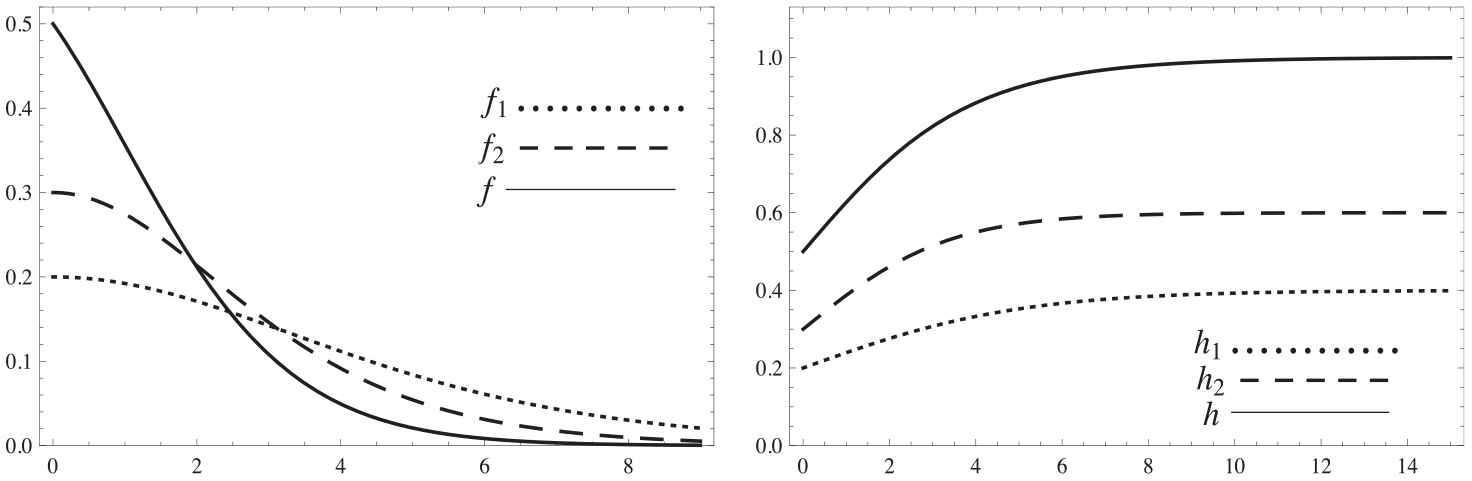
Left (Right) panel: The PDFs (HRFs) of the half-logistic distribution at β1 = 0.4 and β2 = 0.6 with their PDFs(HRFs) under competing risks model.
It may be noticed that Equation (21) can be obtained from (1) by putting
Using Equation (24), the MLP and BPI for
Remark 5.1.
The half-logistic distribution includes one parameter which facilitates the calculations required in the estimation and prediction methods. It has also an advantage rather than the exponential distribution since the first has increasing hazard rate while the latter has constant hazard rate.
6. SIMULATION STUDY AND ILLUSTRATIVE EXAMPLES
6.1. Simulation Study
The following steps are followed to generate progressively type-II censored samples from CDF (21).
For given values of the prior parameters (
where E denotes the expectation andFor given values of
Generate two random samples
Calculate
For given values of the CS
6.2. Simulation Procedure
In this subsection, a Monte Carlo simulation study is carried out in order to determine MLPs and BPIs for
CS1:
which means that we remove one unit after each observed failure of the firstCS2:
which means that we removeCS3:
which means that we removeCS4:
which means that we removeCS5:
which means that we removeCS6:
which means that we remove
Through the simulation procedure, the values
Based on 1000 informative samples, MLPs for
| n* = m* = 10 |
n* = 16 and m* = 10 |
||||||||||
|---|---|---|---|---|---|---|---|---|---|---|---|
| CS | MLP | Bias | MSPE | PI | AIL | MLP | Bias | MSPE | PI | AIL | |
| 1 | 0.2074 | −0.1699 | 0.0952 | (0.0938, 0.3210) | 0.2272 | 0.1364 | −0.1200 | 0.0458 | (0.0618, 0.2109) | 0.1490 | |
| 0.6553 | −0.1538 | 0.1655 | (0.4202, 0.8903) | 0.4701 | 0.4359 | −0.1159 | 0.0840 | (0.2771, 0.5947) | 0.3176 | ||
| 1.1984 | −0.1580 | 0.2800 | (0.8206, 1.5761) | 0.7555 | 0.8713 | −0.1391 | 0.1761 | (0.5904, 1.1523) | 0.5619 | ||
| 1.9042 | −0.2027 | 0.5185 | (1.3437, 2.4646) | 1.1209 | 1.5818 | −0.2235 | 0.4636 | (1.1059, 2.0576) | 0.9518 | ||
| 3.2687 | −0.5587 | 2.1717 | (2.3248, 4.2126) | 1.8878 | 2.9423 | −0.5790 | 2.1348 | (2.0808, 3.8038) | 1.7230 | ||
| 2 | 0.2044 | −0.1676 | 0.0928 | (0.0938, 0.3150) | 0.2212 | 0.1613 | −0.1524 | 0.0732 | (0.0725, 0.2501) | 0.1776 | |
| 0.6535 | −0.1534 | 0.1651 | (0.4223, 0.8847) | 0.4624 | 0.5979 | −0.1582 | 0.1563 | (0.3837, 0.8122) | 0.4285 | ||
| 1.1902 | −0.1570 | 0.2759 | (0.8219, 1.5586) | 0.7367 | 1.1237 | −0.1610 | 0.2653 | (0.7720, 1.4755) | 0.7035 | ||
| 1.8977 | −0.2020 | 0.5142 | (1.3472, 2.4483) | 1.1010 | 1.8550 | −0.2074 | 0.5154 | (1.3183, 2.3917) | 1.0734 | ||
| 3.2552 | −0.5577 | 2.1585 | (2.3404, 4.1700) | 1.8296 | 3.2073 | −0.5602 | 2.1627 | (2.3067, 4.1080) | 1.8013 | ||
| 3 | 0.2059 | −0.1688 | 0.0941 | (0.0924, 0.3195) | 0.2270 | 0.1319 | −0.1160 | 0.0427 | (0.0590, 0.2047) | 0.1457 | |
| 0.6555 | −0.1536 | 0.1656 | (0.4204, 0.8905) | 0.4701 | 0.3850 | −0.1008 | 0.0642 | (0.2445, 0.5255) | 0.2811 | ||
| 1.1930 | −0.1574 | 0.2769 | (0.8148, 1.5711) | 0.7563 | 0.7796 | −0.1549 | 0.1753 | (0.5242, 1.0351) | 0.5109 | ||
| 1.9166 | −0.2041 | 0.5254 | (1.3502, 2.4831) | 1.1329 | 1.5016 | −0.2393 | 0.4711 | (1.0386, 1.9647) | 0.9261 | ||
| 3.2943 | −0.5639 | 2.2038 | (2.3432, 4.2455) | 1.9023 | 2.9263 | −0.5896 | 2.2054 | (2.0529, 3.7997) | 1.7468 | ||
| 4 | 0.2071 | −0.1697 | 0.0956 | (0.0909, 0.3233) | 0.2324 | 0.1321 | −0.1161 | 0.0428 | (0.0583, 0.2059) | 0.1476 | |
| 0.6611 | −0.1550 | 0.1682 | (0.4184, 0.9038) | 0.4854 | 0.3856 | −0.1010 | 0.0647 | (0.2424, 0.5288) | 0.2864 | ||
| 1.1850 | −0.1563 | 0.2741 | (0.8050, 1.5650) | 0.7600 | 0.6730 | −0.0965 | 0.0956 | (0.4522, 0.8938) | 0.4417 | ||
| 1.9130 | −0.2038 | 0.5244 | (1.3457, 2.4804) | 1.1347 | 1.0037 | −0.0970 | 0.1375 | (0.6959, 1.3114) | 0.6156 | ||
| 3.2265 | −0.5529 | 2.1219 | (2.2794, 4.1737) | 1.8942 | 1.3496 | −0.1011 | 0.1855 | (0.9511, 1.7481) | 0.7970 | ||
| 5 | 0.2070 | −0.1696 | 0.0948 | (0.0926, 0.3213) | 0.2287 | 0.1436 | −0.1278 | 0.0521 | (0.0643, 0.2230) | 0.1587 | |
| 0.6579 | −0.1542 | 0.1664 | (0.4218, 0.8940) | 0.4722 | 0.4681 | −0.1219 | 0.0942 | (0.2974, 0.6387) | 0.3412 | ||
| 1.1942 | −0.1574 | 0.2775 | (0.8182, 1.5703) | 0.7520 | 0.8334 | −0.1180 | 0.1447 | (0.5684, 1.0984) | 0.5300 | ||
| 1.9129 | −0.2037 | 0.5227 | (1.3540, 2.4718) | 1.1178 | 1.2810 | −0.1255 | 0.2246 | (0.9010, 1.6610) | 0.7600 | ||
| 3.2281 | −0.5528 | 2.1292 | (2.2968, 4.1594) | 1.8626 | 1.8263 | −0.1527 | 0.3604 | (1.2994, 2.3532) | 1.0539 | ||
| 6 | 0.2079 | −0.1704 | 0.0957 | (0.0927, 0.3266) | 0.2302 | 0.1386 | −0.1224 | 0.0478 | (0.0618, 0.2153) | 0.1535 | |
| 0.6567 | −0.1539 | 0.1663 | (0.4208, 0.8931) | 0.4728 | 0.4335 | −0.1130 | 0.0811 | (0.2748, 0.5922) | 0.3174 | ||
| 1.1750 | −0.1549 | 0.2692 | (0.8049, 1.5451) | 0.7402 | 0.8020 | −0.1210 | 0.1418 | (0.5403, 1.0636) | 0.5232 | ||
| 1.9221 | −0.2047 | 0.5271 | (1.3592, 2.4850) | 1.1258 | 1.3202 | −0.1461 | 0.2625 | (0.9218, 1.7185) | 0.7967 | ||
| 3.2717 | −0.5605 | 2.1771 | (2.3342, 4.2091) | 1.8749 | 2.0127 | −0.2023 | 0.5063 | (1.4302, 2.5952) | 1.1651 | ||
MLPs for
The following steps are followed to determine the AILs and coverage probabilities (COVPs) of BPIs for
Generate a progressively type-II censored random sample under competing risks model as shown in Subsection 6.1. This sample will be called “informative sample.” Based on this sample, calculate BPIs for
Generate another sample (will be called “future sample”) and assign the values of
Repeat the above two steps 1000 times to induce 1000 BPIs for
Calculate the average of the BPIs and hence calculate the AILs of the BPIs.
Calculate the COVPs of the BPIs as follows
The prior parameter values
| n* = m* = 10 |
n* = 16 and n* = 10 |
||||||
|---|---|---|---|---|---|---|---|
| CS | BPI | AIL | COVP | BPI | AIL | COVP | |
| 1 | (0.0503, 1.1472) | 1.0969 | 95.4 | (0.3021, 0.7611) | 0.7290 | 96.1 | |
| (0.2460, 1.9967) | 1.7507 | 95.4 | (0.1660, 1.4125) | 1.2465 | 94.8 | ||
| (0.5349, 2.9466) | 2.4118 | 94.2 | (0.3939, 2.3073) | 1.9134 | 95.2 | ||
| (0.9552, 4.3893) | 3.4341 | 95.7 | (0.7864, 3.9453) | 3.1589 | 95.4 | ||
| (1.7136, 8.2085) | 6.4948 | 95.1 | (1.5304, 7.9319) | 6.4014 | 96.1 | ||
| 2 | (0.0503, 1.1438) | 1.0936 | 95.6 | (0.0403, 0.9910) | 0.9507 | 95.9 | |
| (0.2444, 1.9728) | 1.7283 | 95.7 | (0.2193, 1.8554) | 1.6360 | 94.9 | ||
| (0.5383, 2.9472) | 2.4089 | 94.0 | (0.5097, 2.8744) | 2.3647 | 95.4 | ||
| (0.9607, 4.3864) | 3.4257 | 94.8 | (0.9236, 4.3003) | 3.3767 | 96.6 | ||
| (1.7299, 8.2343) | 6.5044 | 95.9 | (1.6826, 8.1171) | 6.4344 | 95.0 | ||
| 3 | (0.0506, 1.1567) | 1.1061 | 96.0 | (0.0313, 0.7442) | 0.7128 | 96.4 | |
| (0.2454, 1.9937) | 1.7483 | 94.8 | (0.1501, 1.2732) | 1.1231 | 95.0 | ||
| (0.5434, 2.9973) | 2.4540 | 94.8 | (0.3460, 2.1649) | 1.8189 | 94.9 | ||
| (0.9490, 4.3704) | 3.4214 | 96.3 | (0.7366, 3.8634) | 3.1268 | 93.4 | ||
| (1.7089, 8.1976) | 6.4887 | 94.7 | (1.4874, 7.9135) | 6.4262 | 95.6 | ||
| 4 | (0.0506, 1.1604) | 1.1098 | 95.9 | (0.0307, 0.7315) | 0.7008 | 94.1 | |
| (0.2430, 1.9829) | 1.7399 | 95.5 | (0.1472, 1.2538) | 1.1066 | 95.8 | ||
| (0.5422, 3.0050) | 2.4628 | 94.8 | (0.3051, 1.7518) | 1.4467 | 95.4 | ||
| (0.9418, 4.3597) | 3.4179 | 95.0 | (0.5059, 2.3433) | 1.8374 | 95.6 | ||
| (1.7081, 8.2391) | 6.5310 | 96.2 | (0.7673, 3.1182) | 2.3509 | 96.2 | ||
| 5 | (0.0510, 1.1638) | 1.1128 | 95.6 | (0.0349, 0.8324) | 0.7975 | 94.9 | |
| (0.2445, 1.9835) | 1.7390 | 95.0 | (0.1774, 1.4987) | 1.3213 | 96.7 | ||
| (0.5405, 2.9770) | 2.4365 | 93.9 | (0.3800, 2.1550) | 1.7750 | 95.9 | ||
| (0.9524, 4.3757) | 3.4233 | 95.6 | (0.6366, 2.9208) | 2.2842 | 95.7 | ||
| (1.7248, 8.2572) | 6.5323 | 95.2 | (1.0010, 4.0860) | 3.0850 | 95.7 | ||
| 6 | (0.0511, 1.1665) | 1.1154 | 94.0 | (0.0335, 0.7978) | 0.7642 | 95.4 | |
| (0.2428, 1.9702) | 1.7273 | 94.5 | (0.1629, 1.3767) | 1.2139 | 94.7 | ||
| (0.5403, 2.9783) | 2.4380 | 95.2 | (0.3668, 2.1147) | 1.7479 | 95.9 | ||
| (0.9589, 4.4068) | 3.4479 | 94.6 | (0.6592, 3.1088) | 2.4496 | 95.7 | ||
| (1.7203, 8.2415) | 6.5212 | 95.3 | (1.0867, 4.6203) | 3.5335 | 96.4 | ||
The AILs and COVPs of
6.3. Illustrative Examples
6.3.1. Example 1
Based on the values of
Assume that (i)
| 1 | 5.59979 | 5.76755 | 5.59979 | 0.01603 |
| 2 | 1.73549 | 1.63035 | 1.63035 | 0.15559 |
| 3 | 1.38032 | 2.71452 | 1.38032 | 0.18830 |
| 4 | 1.48707 | 2.01749 | 1.48707 | 0.31341 |
| 5 | 8.95048 | 3.23940 | 3.23940 | 0.34363 |
| 6 | 0.48371 | 9.14179 | 0.48371 | 0.41885 |
| 7 | 0.79873 | 1.35164 | 0.79873 | 0.46795 |
| 8 | 5.42455 | 0.57271 | 0.57271 | 0.57271 |
| 9 | 4.07025 | 2.72627 | 2.72627 | 0.70169 |
| 10 | 4.22138 | 3.51768 | 3.51768 | 0.72990 |
| 11 | 2.89722 | 0.15559 | 0.15559 | 0.85833 |
| 12 | 8.68340 | 0.31341 | 0.31341 | 1.00249 |
| 13 | 3.77322 | 3.73408 | 3.73408 | 1.82999 |
| 14 | 1.53726 | 3.16222 | 1.53726 | 2.21175 |
| 15 | 3.17939 | 1.43613 | 1.43613 | 2.22394 |
| 16 | 0.85833 | 1.15286 | 0.85833 | 2.36294 |
| 17 | 5.37478 | 0.41885 | 0.41885 | 3.01668 |
| 18 | 7.13561 | 2.22394 | 2.22394 | 6.14015 |
| 19 | 4.79655 | 1.00249 | 1.00249 | ——— |
| 20 | 4.20190 | 0.70169 | 0.70169 | ——— |
| 21 | 4.63921 | 2.21175 | 2.21175 | ——— |
| 22 | 0.46795 | 1.70203 | 0.46795 | ——— |
| 23 | 2.93812 | 2.36294 | 2.36294 | ——— |
| 24 | 0.34363 | 1.15989 | 0.34363 | ——— |
| 25 | 1.54094 | 0.01603 | 0.01603 | ——— |
| 26 | 6.14015 | 6.22725 | 6.14015 | ——— |
| 27 | 1.82999 | 5.68222 | 1.82999 | ——— |
| 28 | 1.42938 | 0.72990 | 0.72990 | ——— |
| 29 | 3.74519 | 3.01668 | 3.01668 | ——— |
| 30 | 5.85944 | 0.18830 | 0.18830 | ——— |
Informative progressively type-II censored samples. Prior parameter values:
| Ys |
||||||
|---|---|---|---|---|---|---|
| n* | m* | |||||
| 10 | 10 | 0.0520 | 0.8016 | 0.9920 | 1.5103 | 3.7583 |
| 16 | 10 | 0.0520 | 0.6533 | 0.8259 | 1.1179 | 5.8339 |
Selected values for
| n* = m* = 10 |
n* = 16 and m* = 10 |
|||
|---|---|---|---|---|
| MLP | BPI | MLP | BPI | |
| 0.2160 | (0.0525, 1.1930) | 0.1358 | (0.0334, 0.7895) | |
| 0.6818 | (0.2527, 2.0421) | 0.4572 | (0.1687, 1.4314) | |
| 1.2314 | (0.5576, 3.0651) | 0.9021 | (0.4029, 2.3538) | |
| 1.9692 | (0.9986, 4.5919) | 1.6373 | (0.8119, 4.0709) | |
| 3.3635 | (1.8121, 8.7346) | 3.0640 | (1.6033, 8.3531) | |
MLPs and
6.3.2. Example 2
Our object, in this example, is to predict with the (40, 2, 2), (42, 2, 2), (62, 2, 2), (163, 2, 2), (179, 2, 2), (206, 2, 2), (222, 2, 2), (228, 2, 2), (252, 2, 2), (259, 2, 2), (318, 1, 2), (385, 2, 2), (407, 2, 2), (420, 2, 2), (462, 2, 2), (517, 2, 2), (517, 2, 2), (524, 2, 2), (525, 1, 2), (536, 1, 2), (558, 1, 2), (605, 1, 2), (612, 1, 2), (620, 2, 2), (621, 1, 4),
The lifetimes of the mice are assumed to be independent and subject to the exponential distribution in Kundu et al. [32], Weibull distribution in Pareek et al. [33] and Lomax distribution in Cramer and Schmiedt [18].
It can be easily shown that the above progressively type-II censored data could come from CDF (3) with
From the above data and using CDF (3) with
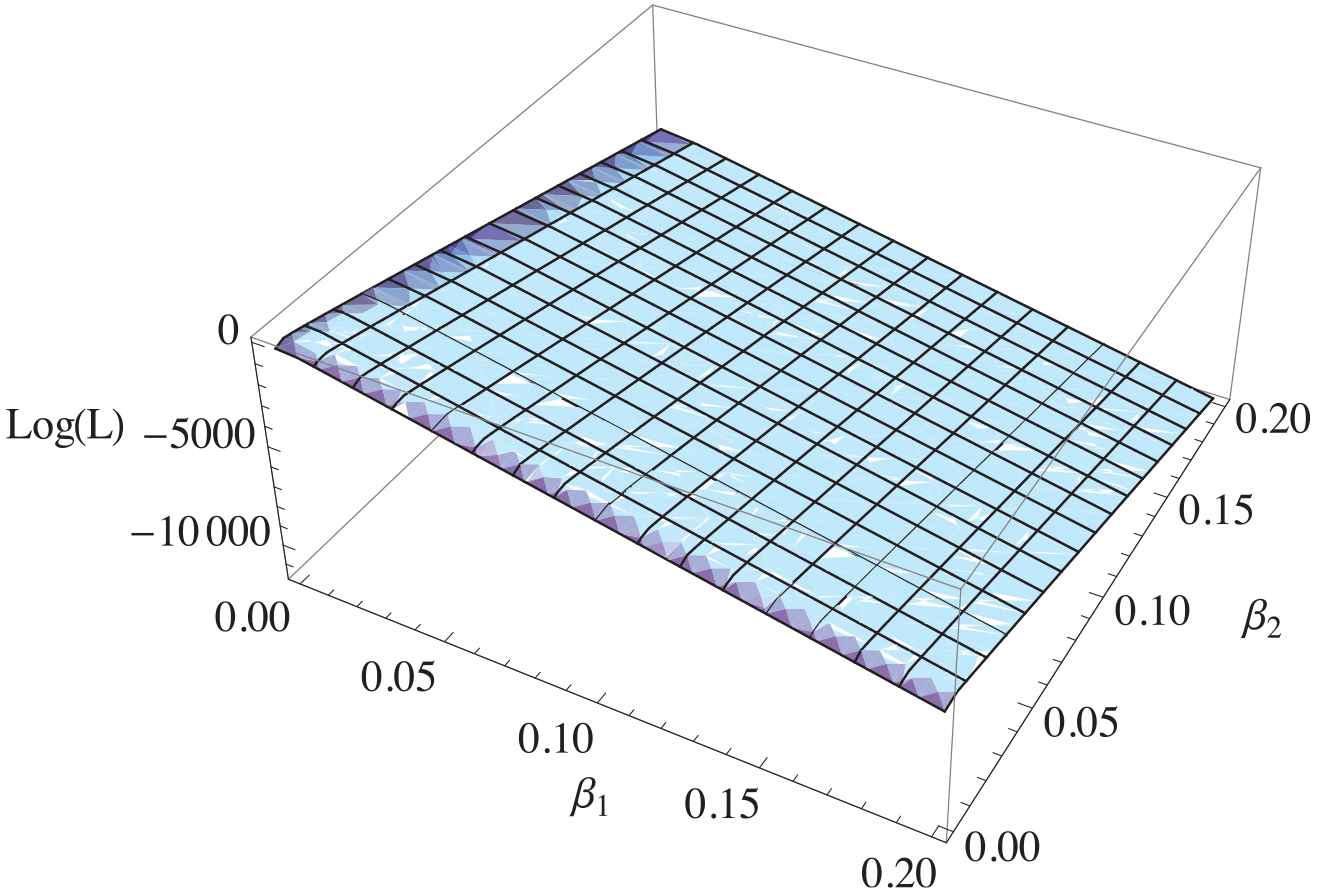
The logarithm of L(β1, β2) under progressively type-II censored competing risks data.
The prior parameter values have been taken to be
| Ys |
||||||
|---|---|---|---|---|---|---|
| n* | m* | |||||
| 10 | 10 | 130.9690 | 413.3470 | 746.4020 | 1193.3700 | 2037.9600 |
| 16 | 10 | 79.5712 | 245.7490 | 425.3320 | 625.3520 | 857.8680 |
MLPs for
| n* = m* = 10 |
n* = 16 and m* = 10 |
|||
|---|---|---|---|---|
| BPI | COVP | BPI | COVP | |
| (31.6553, 703.4732) | 96.0 | (19.4418, 449.9195) | 95.9 | |
| (153.0676, 1197.9496) | 96.7 | (90.4819, 740.9591) | 96.7 | |
| (338.9109, 1792.2874) | 97.1 | (190.2302, 1042.1497) | 97.1 | |
| (608.4114, 2681.1188) | 97.5 | (313.3242, 1378.8600) | 97.5 | |
| (1105.0914, 5116.6316) | 97.2 | (463.0192, 1781.5689) | 97.9 | |
The COVPs in
7. CONCLUDING REMARKS
In this paper, under competing risks model and based on a progressively type-II censored informative sample generated from the half-logistic distribution, we have discussed MLPs and BPIs for future progressively type-II censored competing risks data from the same population. An illustrative example based on simulated data and another one based on real data have been considered to investigate the performance of prediction.
From Table 1 we observe the following:
For all considered CSs, by increasing the index
In the fourth column in which we have considered the progressive censoring in future sample, the MSPEs and AILs give less values with respect to the last three CSs than those for the above CSs (CS1, CS2, CS3).
From Table 2 we observe the following:
The COVPs of the BPIs are quite close to the nominal confidence levels
For all considered CSs, by increasing the index
In the fourth column in which we have considered the progressive censoring in future sample, better results for the BPIs, through smaller values for the AILs and closer values for the COVPs (near to
CS4, in which we remove all the surviving units after the last failure, gives better results with respect to the AILs, than the other CSs.
Numerical computations show that the above results do not change by changing the values of the prior parameters.
If the hyperparameters are unknown, “simple empirical Bayes estimators” may be obtained by using “past samples,” see [34]. Alternatively, one could use hierarchical Bayes approach in which a suitable prior for the vector of hyperparameters is used, see [35].
CONFLICT OF INTEREST
Essam. K. AL-Hussaini contributes with the review of the paper. Alaa H. Abdel-Hamid contributes with the idea and preparation of the paper. Atef. F. Hashem contributes with derivation (calculation) of the analytical (numerical) results in addition to writing the paper.
REFERENCES
Cite this article
TY  - JOUR
AU  - Essam K. AL-Hussaini
AU  - Alaa H. Abdel-Hamid
AU  - Atef F. Hashem
PY  - 2020
DA  - 2020/03/05
TI  - Prediction for Progressively Type-II Censored Competing Risks Data from the Half-Logistic Distribution
JO  - Journal of Statistical Theory and Applications
SP  - 36
EP  - 48
VL  - 19
IS  - 1
SN  - 2214-1766
UR  - https://doi.org/10.2991/jsta.d.200224.004
DO  - 10.2991/jsta.d.200224.004
ID  - AL-Hussaini2020
ER  -