
Finite Mixture Modeling via Skew-Laplace Birnbaum–Saunders Distribution
- DOI
- 10.2991/jsta.d.200224.008How to use a DOI?
- Keywords
- Birnbaum–Saunders distribution; Normal mean-variance mixture model; Skew-Laplace distribution; Finite mixture model; ECM algorithm
- Abstract
Finite mixture model is a widely acknowledged model-based clustering method for analyzing data. In this paper, a new finite mixture model via an extension of Birnbaum–Saunders distribution is introduced. The new mixture model provide a useful generalization of the heavy-tailed lifetime model since the mixing components cover both skewness and kurtosis. Some properties and characteristics of the model are derived and an expectation and maximization (EM)-type algorithm is developed to compute maximum likelihood estimates. The asymptotic standard errors of the parameter estimates are obtained via offering an information-based approach. Finally, the performance of the methodology is illustrated by considering both simulated and real datasets.
- Copyright
- © 2020 The Authors. Published by Atlantis Press SARL.
- Open Access
- This is an open access article distributed under the CC BY-NC 4.0 license (http://creativecommons.org/licenses/by-nc/4.0/).
1. INTRODUCTION
The Birnbaum–Saunders (BS) distribution [1,2] is a positively skewed and unimodal distribution with non-negative support. The BS distribution has recently received considerable attention in the literature of statistics including lifetime, survival and environmental data analysis (see, e.g. [3–6]). An important property of the BS distribution is that it is closely related to the normal distribution by means of a simple stochastic representation. A random variable
Recently, some generalizations and extensions of the BS distribution have been proposed through replacing the standard normal variable
Another important family of skewed distributions is the class of normal mean-variance (NMV) mixture models [13]. Concerning the asymmetric properties of the NMV models, Arslan [14] introduced the skew-Laplace (SL) distribution via considering the inverse gamma distribution as a mixing random variable. Arslan also developed the expectation and maximization (EM) algorithm [15] for computing maximum likelihood (ML) estimates.
In reliability studies, data often arise from heterogeneous populations and so they need to be modeled by a mixture of two or more life distributions. The finite mixture of distributions (FM) is a finite convex linear combination of distribution functions which is also useful to approximate complicated probability densities presenting multimodality. A comprehensive survey of the FM models can be found in [16,17]. Because of the usefulness of the FM models in reliability, different kinds of the lifetime mixture models have been recently proposed. Ali [18] introduced a mixture of the inverse Rayleigh model for lifetime study in engineering processes and studied different properties of the proposed model. Balakrishnan et al. [19] proposed three different mixture models based on the BS distribution as (a) mixture of two different BS distributions, (b) mixture of a BS distribution and a length-biased version of another BS distribution and (c) mixture of a BS distribution and its length-biased version.
Due to the asymmetric properties and robustness of the SL distribution, the main objective of this paper is to propose a
The remainder of the paper is unfolded as follows. In Section 2, we briefly review the univariate SL distribution and some of its properties. We also present the skew-Laplace Birnbaum–Saunders (SLBS) distribution with its characteristics in this section. Section 3 describes the finite mixture model of the proposed SLBS distribution and develops the EM-type algorithm for estimating parameters. In Section 4, we analyze a real data set for the purpose of illustrating the performance of the proposed mixture model. Two simulation studies are carried out to verify the robustness of the new model and to check finite-sample properties of the ML estimates in Section 5. Finally, the paper is closed with a short summary in Section 6.
2. PRELIMINARIES
A random variable
Proposition 2.1.
The skewness and kurtosis of
Proof.
The results are straightforward by using representation (3).
Figure 1 displays the curves of skewness and kurtosis of the SL distribution. It can be observed that the SL distribution takes wider ranges of skewness and kurtosis as compared with the skew-normal distribution. In the following, the notation
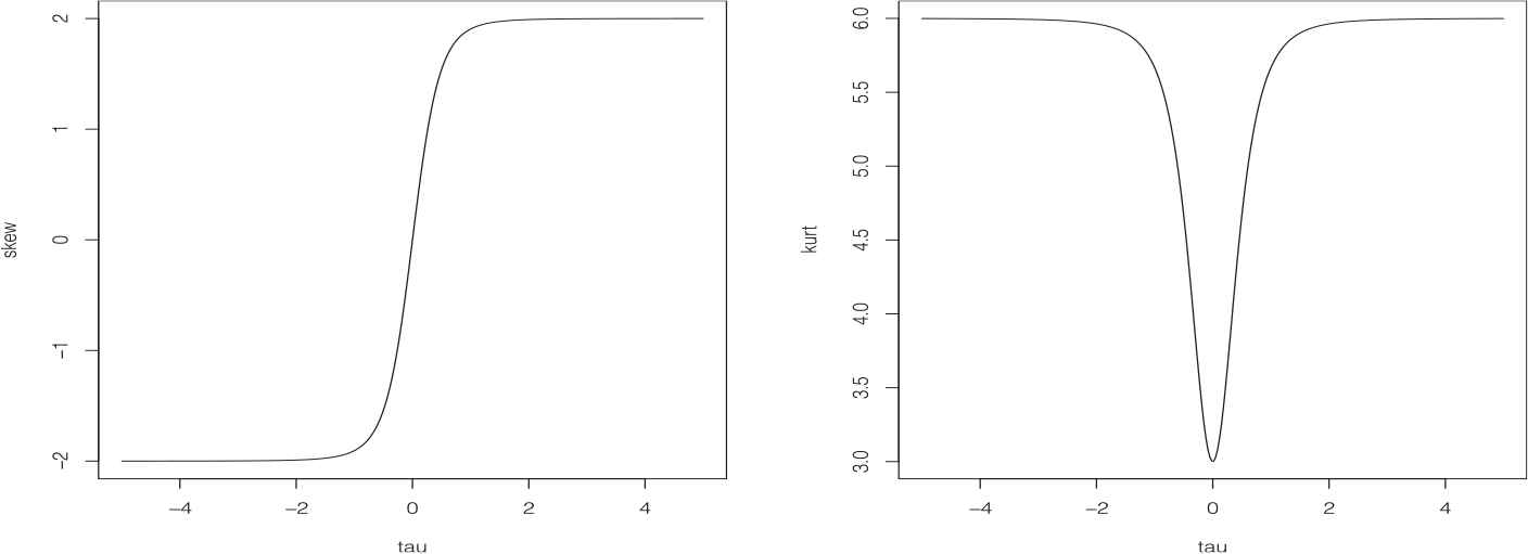
The skewness and kurtosis plots of the skew-Laplace (SL) distribution.
Replacing
This model will be denoted by
Theorem 2.1.
Some properties of the SLBS distribution are as follows:
The density of SLBS distribution tends to the density of Laplace BS distribution, as
The random variable
If
Let
Using the “
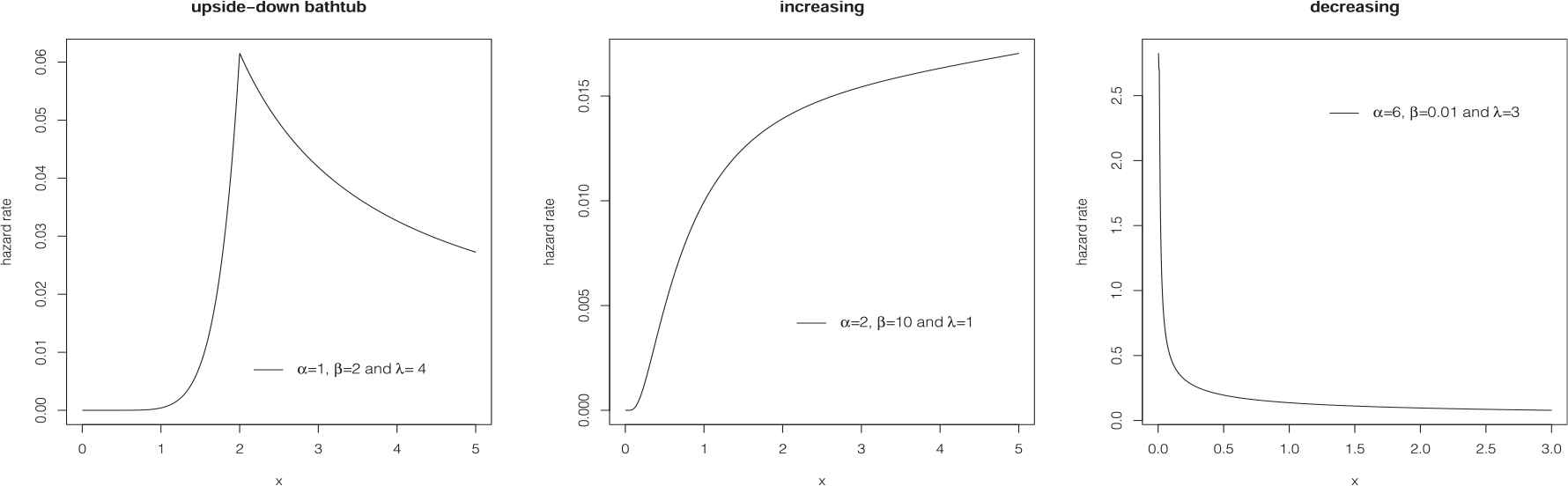
The hazard rate plots of the skew-Laplace Birnbaum-Saunders (SLBS) distribution for some parameter values.
Now in the following theorem, we present a transformational result for the random variable
Theorem 2.2.
Let
Remark 2.1.
As a measure of the uncertainty or randomness of a system, the entropy plays an important role in many sciences. The entropy has been used in the various situations and its numerous measures have been studied and compared in the literature. For a random variable
There is no a closed-form expression for the integral and expectations. Hence, Theorems 2.1 and 2.2 are useful to compute them numerically.
Consequently, we establish the following proposition and theorem, which are useful for obtaining the complete log-likelihood function and for the calculation of some conditional expectations involved in the proposed EM-type algorithm discussed in the next section.
Proposition 2.2.
Let
Theorem 2.3.
Let
Proof.
By Bayes' rule, the conditional distribution is simply obtained. Moreover, the conditional expectation can be derived by using properties of the GIG distribution and the Bessel function, see [22].
3. FINITE MIXTURE OF THE SLBS DISTRIBUTIONS
Consider
The ML estimate of the parameters involved in (7) can be obtained directly. However, maximization of (7) is complicated. Another approach for getting ML estimator is the EM algorithm. In this approach, the idea is to solve tractable complete log-likelihood problems repeatedly instead of solving a difficult incomplete log-likelihood problem. For applying this approach to Mix-SLBS model, it is convenient to construct a log-likelihood function by introducing a set of allocation variables
Therefore, the complete data log-likelihood function for
3.1. Parameter Estimation via ECM Algorithm
To compute the ML estimate of the unknown parameters involved in (8), we adopt the Expectation Conditional Maximization (ECM) algorithm [23]. The ECM algorithm is a variant of the EM algorithm with the maximization (M) step of EM replaced by a sequence of computationally simpler conditional maximization (CM) steps. The ECM algorithm for ML estimation of the Mix-SLBS proceeds as follows:
E-step: At the iteration
whereCM-steps: Put
where
The above procedure is iterated until a suitable convergence rule is satisfied. To avoid an indication of lack of progress of the algorithm [24], we recommend adopting the Aitken acceleration [25] method as the stopping criterion. To apply this approach, the asymptotic estimate of the log-likelihood [16] is computed by
3.2. Estimation of Standard Errors
To compute the asymptotic covariance of the ML estimates
As a result, the standard errors of
4. REAL DATA ANALYSIS
In this section, we use Enzyme data to illustrate the performance of the Mix-SLBS model to fit the data. These data, originally analyzed by Bechtel et al. [28], correspond to the enzymatic activity in the blood and represent the metabolism of carcinogenic substances among 245 unrelated individuals. The enzymatic activity is quantified by the molar ratio between two metabolites of caffeine. Bechtel et al. concluded that a mixture of two skewed distributions is suitable for analyzing these Enzyme data. Recently, Balakrishnan et al. [19] used these data to compare three kinds of BS mixture model. Their proposed model were (a) mixture of two BS distribution (Mix-BS), (b) Mixture of Length-biased BS and BS distributions (Mix-LBBS) and (c) Mixture of Length-biased BS and BS distributions with the same parameters (Mix-LBSBS). Here, the Akaike Information Criterion (AIC) [29] as well as the Bayesian Information Criterion (BIC) [30] are computed to identify the best selected model for comparing our proposed model with these three models. The AIC and BIC are formulated by
We fit Mix-SLBS model for different number of components
| Mix-SLBS |
Mix-BS |
Mix-LBBS |
Mix-LBSBS |
|||||
|---|---|---|---|---|---|---|---|---|
| Parameter | MLE | SE | MLE | SE | MLE | SE | MLE | SE |
| 0.636 | 0.007 | 0.629 | 0.031 | 0.450 | 0.028 | 0.417 | 0.026 | |
| 0.399 | 0.001 | 0.533 | 0.032 | 0.365 | 0.034 | 1.038 | 0.084 | |
| 0.185 | 0.012 | 0.175 | 0.007 | 0.171 | 0.007 | 0.216 | 0.012 | |
| −0.029 | 0.001 | – | – | – | ||||
| 0.210 | 0.016 | 0.319 | 0.025 | 1.274 | 0.114 | 1.038 | 0.084 | |
| 1.003 | 0.039 | 1.274 | 0.043 | 0.213 | 0.044 | 0.216 | 0.012 | |
| 0.587 | 0.003 | – | – | – | ||||
| −46.394 | −59.168 | −71.091 | −115.899 | |||||
| AIC | 106.787 | 128.336 | 152.182 | 237.798 | ||||
| BIC | 131.296 | 145.842 | 169.688 | 248.302 | ||||
| KS | 0.039 | 0.053 | 0.111 | 0.151 | ||||
| p-value | 0.832 | 0.507 | 0.005 | |||||
BS, Birnbaum–Saunders; LBBS, Length-biased Birnbaum–Saunders; LBSBS, Length-biased Birnbaum–Saunders and Birnbaum–Saunders distributions with the same parameters; MLE, maximum likelihood estimation; SE, standard error; SLBS, skew-Laplace Birnbaum-Saunders.
The bold numbers are related to the best model coordinating to the each model comparison measure.
Parameter estimates with corresponding standard errors of the Enzyme data set.
On the other hand, the
Finally, we provide the probability-probability (PP)-plot of the two best fitted models in Figure 3. The PP-plot shows that the Mix-SLBS model adapts to the shape of the histogram very accurately.
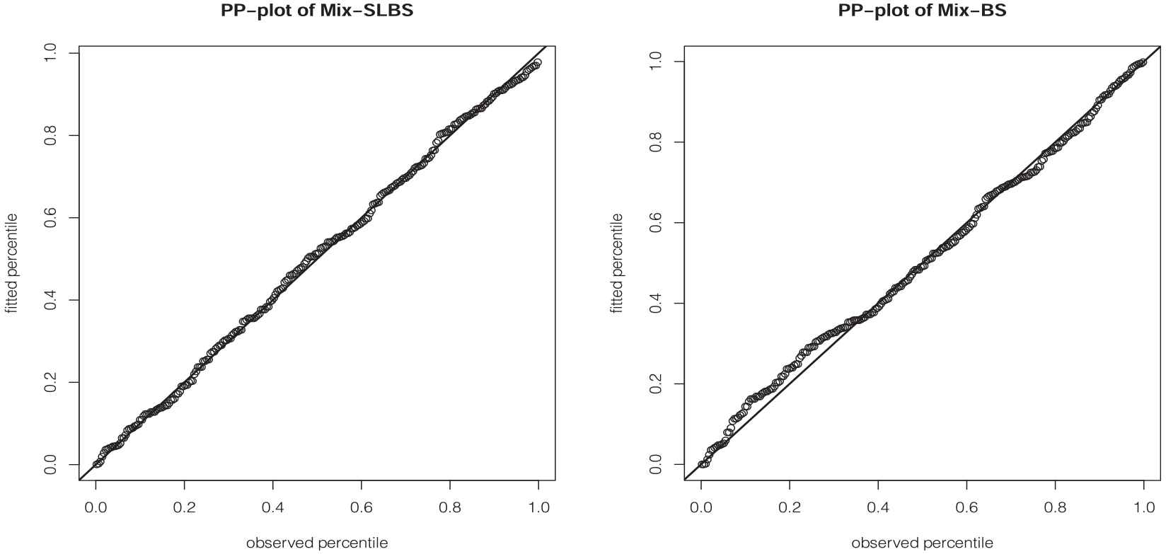
The PP-plots of two best distributions.
5. SIMULATION STUDY
In this section, we conduct two simulation studies in order to examine the performance of the proposed method. The first study shows that the underlying Mix-SLBS model is robust in the ability to cluster heterogeneous lifetime data in the presence of outliers. In the second simulation study, we investigate if the ML estimates obtained using the proposed ECM algorithm can provide good asymptotic properties. All simulation studies are done in the statistical software R.
5.1. Robustness of the Model
In the first experiment, the ability of the Mix-SLBS model in clustering observations (allocating them into groups of observations that are similar in some sense) is verified. Although, we know that each data point belongs to one of
We generated 500 samples from a mixture of two BS and two SLBS densities with the parameter values at
Table 2 shows the mean value of
| S1: Fitted Model |
S2: Fitted Model |
||||
|---|---|---|---|---|---|
| True Model | Sample Size | Mix-BS | Mix-SLBS | Mix-BS | Mix-SLBS |
| Mix-BS | 100 | 0.8134 | 0.7861 | 0.7998 | 0.7460 |
| 500 | 0.8231 | 0.8350 | 0.8067 | 0.7984 | |
| 1000 | 0.8358 | 0.8345 | 0.8109 | 0.8201 | |
| Mix-SLBS | 100 | 0.5189 | 0.9722 | 0.6018 | 0.8874 |
| 500 | 0.4477 | 0.9761 | 0.5929 | 0.9146 | |
| 1000 | 0.4449 | 0.9776 | 0.5901 | 0.9191 | |
BS, Birnbaum–Saunders; SLBS, skew-Laplace Birnbaum-Saunders.
Mean right allocations rates for fitted models.
5.2. Asymptotic Properties
We carry out a second simulation study to check the finite-sample performances of the ML estimates obtained by using the ECM algorithm. To show the effect of parameters on the estimation procedure, we consider three set of the parameter values
As suggested in [32], the parameters were taken to produce highly skewed and heavy-tailed distributions. In each replication of 500 trials, we generate data of size
Table 3 presents the results of the simulation. It is evident that both magnitudes bias and MSE of the estimators decrease and tend to toward zero when the sample size increases. It shows that the ML estimates obtained via the ECM algorithm are empirically consistent.
| S1 |
S2 |
S3 |
|||||||||||
|---|---|---|---|---|---|---|---|---|---|---|---|---|---|
| Measure | Parameter | Sample Size |
Sample Size |
Sample Size |
|||||||||
| 100 | 250 | 500 | 1000 | 100 | 250 | 500 | 1000 | 100 | 250 | 500 | 1000 | ||
| R.Bias | 0.237 | 0.034 | 0.024 | 0.017 | 0.211 | 0.097 | 0.046 | 0.026 | 0.030 | 0.020 | 0.022 | 0.001 | |
| 0.450 | 0.372 | 0.284 | 0.108 | 0.445 | 0.397 | 0.308 | 0.134 | 0.296 | 0.176 | 0.098 | 0.038 | ||
| 0.182 | 0.134 | 0.110 | 0.094 | 0.195 | 0.114 | 0.054 | 0.009 | 0.084 | 0.066 | 0.062 | 0.007 | ||
| 0.098 | 0.089 | 0.069 | 0.043 | 0.984 | 0.569 | 0.327 | 0.209 | 0.247 | 0.209 | 0.150 | 0.095 | ||
| 0.456 | 0.369 | 0.301 | 0.198 | 0.365 | 0.259 | 0.186 | 0.097 | 0.080 | 0.025 | 0.008 | 0.002 | ||
| 0.557 | 0.457 | 0.311 | 0.167 | 0.399 | 0.279 | 0.153 | 0.068 | 0.527 | 0.473 | 0.335 | 0.196 | ||
| 0.209 | 0.094 | 0.045 | 0.013 | 0.188 | 0.078 | 0.026 | 0.009 | 0.219 | 0.208 | 0.189 | 0.163 | ||
| MSE | 0.050 | 0.027 | 0.012 | 0.005 | 0.059 | 0.034 | 0.017 | 0.008 | 0.058 | 0.043 | 0.031 | 0.024 | |
| 0.053 | 0.034 | 0.026 | 0.015 | 0.444 | 0.219 | 0.134 | 0.086 | 0.256 | 0.185 | 0.099 | 0.010 | ||
| 0.156 | 0.089 | 0.055 | 0.019 | 0.201 | 0.152 | 0.091 | 0.032 | 0.113 | 0.066 | 0.043 | 0.009 | ||
| 0.009 | 0.009 | 0.008 | 0.006 | 1.628 | 1.079 | 0.793 | 0.258 | 0.062 | 0.040 | 0.015 | 0.001 | ||
| 0.331 | 0.218 | 0.161 | 0.083 | 0.242 | 0.173 | 0.109 | 0.045 | 0.049 | 0.023 | 0.014 | 0.008 | ||
| 1.654 | 1.202 | 0.985 | 0.384 | 0.887 | 0.496 | 0.273 | 0.129 | 0.691 | 0.467 | 0.323 | 0.165 | ||
| 1.029 | 0.504 | 0.321 | 0.176 | 0.835 | 0.638 | 0.356 | 0.192 | 0.612 | 0.412 | 0.361 | 0.136 | ||
EM, expectation and maximization; MSE, mean squared error.
Bias and mean squared errors for EM estimates of simulated data.
6. CONCLUSIONS
In this paper, we have dealt with a new finite mixture model based on a new extension of BS distribution, called the Mix-SLBS. We have presented a convenient hierarchical representation and developed the ECM algorithm to obtain the ML estimates of the parameters. Numerical results suggest that the proposed Mix-SLBS distributions is well suited to the experimental data and can be more robust and flexible against outliers as compared with the 3 mixture competitors, proposed by Balakrishnan et al. [19].
Some possible directions of the current work remain that deserve further attention. For instance, the linear and non-linear regression model based on the SLBS distribution can be presented by using Theorem 2.2 [33,34]. As another extension of this work, it is worthwhile to generalize BS distribution in more general case by considering GIG distribution instead of
CONFLICT OF INTEREST
No potential conflict of interest was reported by the authors.
AUTHORS' CONTRIBUTIONS
M. Naderi developed main methodological parts of the paper whereas M. Mozafari and K. Okhli implemented the methodology in the R program and applied them to the real and simulated data examples.
ACKNOWLEDGMENTS
We are grateful to the Editor-in-Chief, anonymous referees for their comments, which greatly improved this work. M. Naderi is also appreciate the support by the National Research Foundation, South Africa (Reference: CPRR160403161466 351 Grant No. 105840, SARChI Research Chair- UID: 71199, and STATOMET).
REFERENCES
Cite this article
TY  - JOUR
AU  - Mehrdad Naderi
AU  - Mahdieh Mozafari
AU  - Kheirolah Okhli
PY  - 2020
DA  - 2020/03/05
TI  - Finite Mixture Modeling via Skew-Laplace Birnbaum–Saunders Distribution
JO  - Journal of Statistical Theory and Applications
SP  - 49
EP  - 58
VL  - 19
IS  - 1
SN  - 2214-1766
UR  - https://doi.org/10.2991/jsta.d.200224.008
DO  - 10.2991/jsta.d.200224.008
ID  - Naderi2020
ER  -