Nakagami distribution; Selection model; Distribution theory; Moment generating function; Log-likelihood function; Monte Carlo simulation
Abstract
In this article, a selection of Nakagami distribution is investigated. Some properties of the model with some plots of the density function are illustrated. Additionally, weighted of the one-sided Gaussian distribution, Generalized Rayleigh distribution are discussed as a special case of Generalized Nakagami distribution. In addition, maximum likelihood estimators are investigated with numerical methods and are compared by four sub-models with a real wave height data set. Finally, a simulation study is presented for parameters.
Nakagami distribution (NA) is useful for modeling the fading of radio signals and other areas of telecoms engineering. It has the applications in medical imaging investigation to model the ultrasounds especially in Echo (heart efficiency test). It is also helpful for modeling high-frequency seismogram envelopes. The reliability theory also make wide use of the NA distribution. By reason of the memory less property of this distribution, it is well appropriate to model the constant hazard rate portion; as it is used in reliability theory. Also, it is also used in the study of failure times of electrical components. On the other hand, the NA distribution is the excellence distribution to check the reliability of electrical component as compared to Gamma, Weibull and lognormal distributions.
The random variable X has the NA distribution if its probability density function is defined as follows:
gxμ,Ω=2μ∕Ωμx2μ−1exp−μx2∕Ω∕Γμ,μ>0;Ω>0,x>0,(1)
where μ is a shape parameter and Ω is a second parameter controlling spread (scale parameter). The cumulative distribution of a random variable from (1) can be obtained as
G(x|μ,Ω)=1Γ(μ)γ(μ,μx2∕Ω),(2)
where γ.,. is the incomplete gamma function. In Telatar [1], Gxμ,Ω is represented in terms of an incomplete gamma function dependent on the average signal-to-noise ratio (μx2∕Ω) which we denoted by ASNR. This allows the system to be characterized. The NA distribution covers a wide range of fading conditions. A special case of the NA distribution in which μ=0.5 implies the one-sided Gaussian distribution (OG). Also, when μ=1, it implies the Rayleigh distribution RA. In addition, if Y belongs to gamma distribution with shape and scale parameters θ1 and θ2 respectively, then Y belongs to NA distribution with parameters μ=θ1 and Ω=θ1θ2. Finally, if 2μ is integer-valued and if B follows a chi distribution with parameters 2μ, hence Ω∕2μB∈gxμ,Ω.
The problem of modeling lifetime of systems and components in reliability theory and survival analysis among other sciences is very important. In some real situations the measurements are not reported according to the standard distribution of the data. This may be due to the fact that the units of a population have unequal chances in order to be recorded by investigator. In a special case, the probability of recording data from the main population depends on size (length) of the data. The random sample drawn in this way is called a size-biased sample.
In this article, we pay attention to a selection model from the NA distribution. Selection distributions have been considered extensively by many authors; for a best survey of estimation method discussions and applications, see Heckman [2], Copas and Li [3], Arrellano-Valle et al. [4], Signer et al. [5], Balakrishnan et al. [6], Zamani et al. [7] and Arashi et al. [8] and more recently. The organization of this paper is as follows: In Section 2, we present definition and some representations of this model. In Section 3, some important properties are discussed. Also, numerical methods and graphs helped to picture some measures are obtained. Statistical inferences by numerical methods are fulfilled in Section 4 to estimate the parameters of the introduced distribution with real wave height data. In Section 5, the explanation of various estimators compared by performing the Monte Carlo simulation is studied.
We use the notation X→DY to mean that X and Y are equal in distribution.
2. DEFINITION
Let A∈R+ and B∈R+ be two random vectors and D to be a measurable subset of R+. Arellano-Valle et al. [4] studied a weighted distribution as the conditional distribution of B given A∈D. Clearly, a p–dimensional random vector Xw is said to have a multivariate weighted density function with parameters depending on the characteristics of A, B and D, if Xw→DBA∈R. If B has a pdf, fB, then Xw has a pdf as follows:
fXwx=fBxPrA∈DB=xPrA∈D.(3)
The random variable Xw is called the weighted version of X, and its distribution in relative to X is called the weighted distribution of X with weight function wx. Some special weighted functions are mentioned in Patil [9] and Azzalini [10].
Let X be a random variable with the probability density function (1) and let we selected generalized weighted function as mentioned in Patil [9] as
As mentioned in Gradshteyn and Ryshik [11], we know that the lower incomplete gamma function can be rewritten as
γα,x=xαα×1F1α;1+α;−x,
According to Gradshteyn and Ryshik [11] α and x are parameters and 1F1.;.;. is the generalized hypergeometric function with one parameter of type 1 and one parameter of type 2. Suppose for a reasonably low outage probability, the ASNR has to be sufficiently large, that is, the term μx2∕Ω in (2) has to be small, we invoke an asymptotic expansion of the confluent hypergeometric function at small x. From the series expansion in Gradshteyn and Ryshik [11], we observe that 1F1α;1+α;−x→1 for x→0. By taking γμ,μx2∕Ω∕Γμ=u, we get that (5) can be expressed as
Ii,j,θμ,Ω=Ωμθ2Γμ+1θ2μBj+1,i+θ2μ+1,(6)
whereas B.,. is beta function. By using (4) and (6), and after some elementary algebra, we have Generalized Nakagami density function, GN, (denoted as GNi,j,θ,μ,Ω) as follows:
fXwx=φ1μ,θ,Ωφ2−1μ,θ,Ω,x>0,(7)
where
φ1μ,θ,Ω=2γμ,μx2∕ΩΓμ−γμ,μx2∕Ωjx2μ+θ−1exp−μx2∕Ω;
φ2μ,θ,Ω=Ωθ2+μμθ1−μ−2μ22μΓi+j+θ2μ+1μBj+1,i+θ2μ+1.
In addition, we can conclude that a generalized OG distribution (denoted as fXw[1](x)) and a Generalized RA distribution (denoted as fXw[2](x)) as sub-models of (7) as respectively follows:
fXw[1](x)=π−j+θ+12φ3(μ,θ,Ω)φ4−1(μ,θ,Ω),x∈R+,
and
fXw[2](x)=φ4−1(μ,θ,Ω)φ5(μ,θ,Ω),x∈R+,
where erfx is error function,
φ3μ,θ,Ω=2θ+12erfx1∕2Ωiπ−πerfx1∕2Ωjxθexp−x2∕2Ω,
φ4μ,θ,Ω=Ωθ+12Bj+1,i+θ+1 and
φ5μ,θ,Ω=2γ1,x2∕Ωi1−γ1,x2∕Ωjxθ+1exp−x2∕Ω.
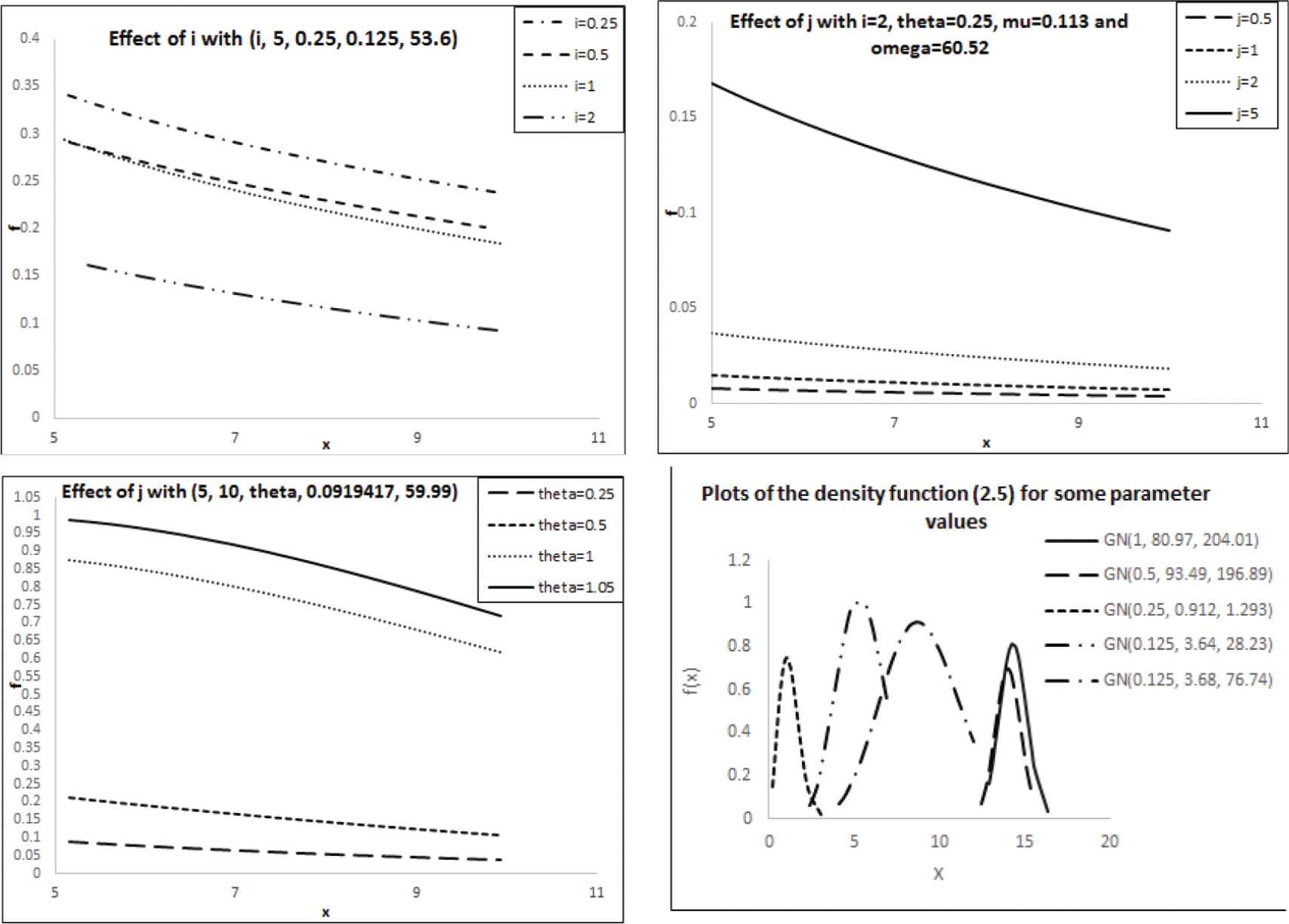
Now, we consider the effect of any parameter on the pdf of GNi,j,θ,μ,Ω introduced in (7) with Figure 1. In each panel, one of the parameters changes in first three panels and in the last panel we change all parameters with together.
Figure 1
Plots of the density function with effect of parameters.
We furnish two simple formula for pdf of the GNi,j,θ,μ,Ω distribution, if j∉ℤ>0 or j∈ℤ>0. First, if |x|<1 and j∉ℤ+, it follows the series (Nadarajah and Kotz [12], p. 324, Eq. (1.7))
(1−x)j=∑y=0∞(−1)yΓ(j+1)Γ(j−y+1)y!xy.(8)
Using the series representation (8), the pdf of the GNi,j,θ,μ,Ω distribution for |γμ,μx2∕Ω∕Γμ|<1 and j∉ℤ+ can be expanded as
where cμ,j,in,k=μnn!μ+1nnΩ∕μμk+i+μ+θ2+n2μk+i+μ+θ2+n2−1!.
3. PROPERTIES OF THE GN DISTRIBUTION
We need to emphasize the importance of hazard rate, reversed hazard rate, moments and moment generating functions in any statistical analysis especially in applied issues. An advantages and characteristics of a distribution can be studied through measures of central tendency; dispersion functions; measures of skewness and kurtosis.
The hazard rate rx=fXwx∕1−FXwx, and reversed hazard rate functions r̃x=fXwx∕FXwx of GNi,j,θ,μ,Ω can be obtained directly using Equations (10–12, 14).
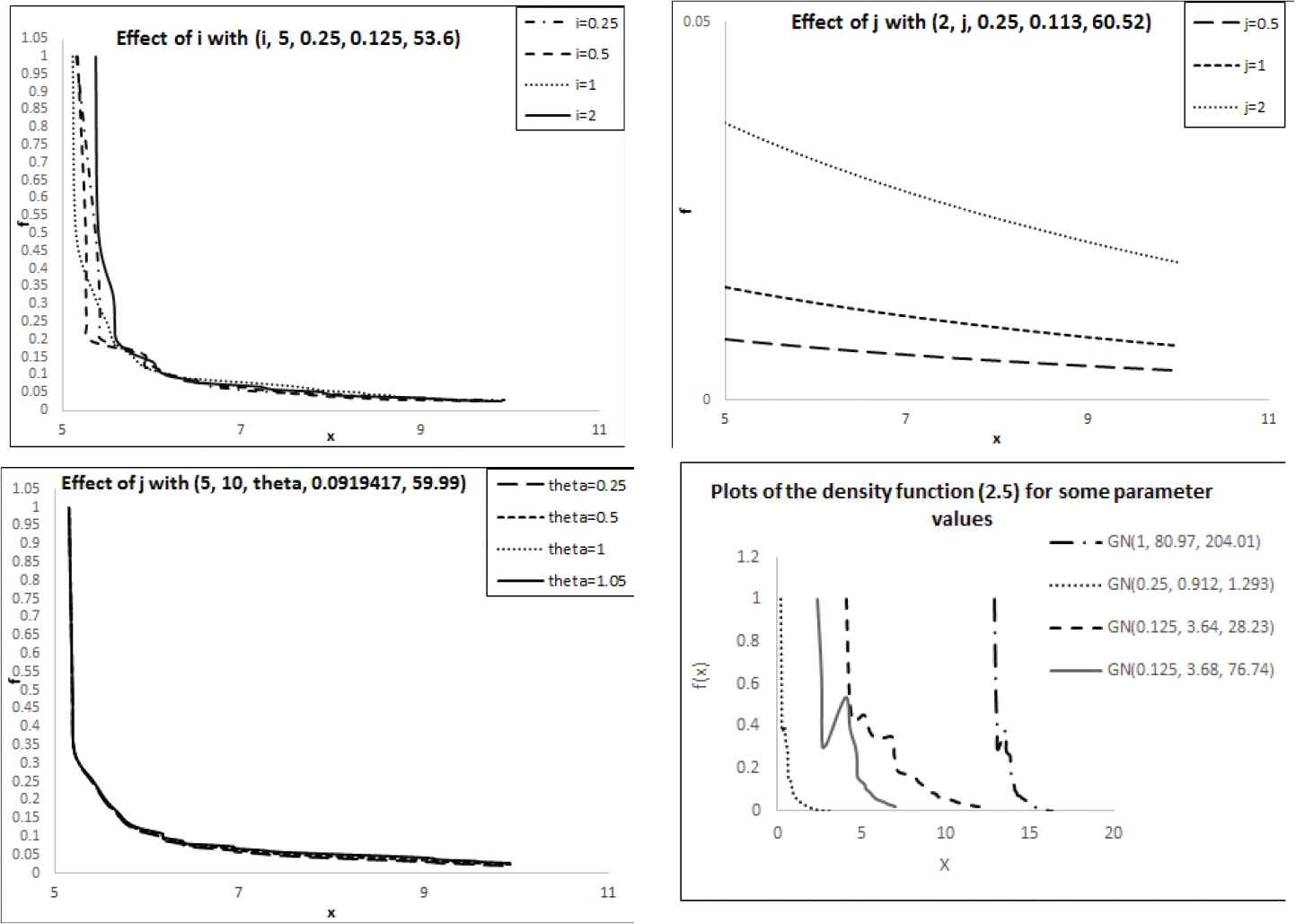
Now, we consider the effect of any parameter on reversed hazard function with Figure 2. In each panel, one of the parameters is changed.
Figure 2
Plots of reversed hazard function with effect of parameters.
where ϖ¯μ,j,i(n,k)=ϖμ,j,i(n,k)((μ)n∕(n!(μ+1)n))n∕([(μ∕Ω)]μ(k+i)+μ+θ2+n2Ii,j,θ(μ,Ω)). Now, The skewness and kurtosis measures can be obtained from the ordinary moments utilizing well-known relationships.
If X~GNi,j,θ,μ,Ω, then its moment generating function is given by
These central indices computed numerically, and we show output for some values that indicate in the Table 1 as
(θ,μ,Ω)
Mean
Median
Mode
(1, 80.97, 204.01)
14.2838
14.1990
14.2357
(0.5, 93.49, 196.89)
14.0072
13.9790
14.0198
(0.25, 0.912, 1.293)
1.0091
0.9493
1.0548
(0.125, 3.68, 76.74)
5.4827
5.4178
4.9304
(0.125, 3.64, 28.23)
8.9588
8.8974
8.6173
Table 1
The mean, median and mode of GNθ,μ,Ω.
The basic uncertainty measure for density function f is differential entropy
HX(f)=E[−lnfX(X)]=∫0∞fX(x)ln1fX(x)dx.
The differential entropy of a non-negative absolutely continuous random variable X, is also known as Shannon information measure or sometime called dynamic measure of uncertainty. Intuitively speaking the entropy gives the expected uncertainty contained in fx about the predictability of an outcome of X, see Ebrahimi and Pellerey [14]. It also measure how the distribution spreads over its domain. A high value of HX corresponds to a low concentration of the probability mass of X.
When θ=1,i=j=0, the density function in (7) is referred to as length-biased distribution. Then, we have
Exθ=1ΓμΩμθ2Γμ+θ2.
Hence,
HXfXwx=ln2+μ+θ2lnμ∕Ω−1+2μ+θ−12ψμ+θ2−lnμΩ−lnΓμ+θ2,
where
∫0∞tv−1lntexp−ptdt=Γvp−vψv−lnp.
Also, Havrda and Charvat [15] introduced β–entropy class as follows:
In this section, we consider the problem of statistical inference about generalized weighted of the NA distribution such as maximum likelihood estimator (MLE) of the unknown parameters, asymptotic distribution and bootstrap confidence intervals and bias reduced maximum likelihood.
4.1. MLE and Asymptotic Distribution
Let X1,X2,…,XN be random variables that are i.i.d. according to (7) and Θ=i,j,θ,μ,ΩT. The log-likelihood function of the independent multivariate generalized weighted of the NA distribution based on X1,X2,…,XN is given by
where xk,k=1,…,N are samples of Xk,k=1,…,N, and we simply apply the chain rule:
∂∂xlnΓx+k=−γ+∑r=1∞1r−1r+x+k−1,
where γ is the Euler–Mascheroni constant. Let Cu=μμ−1xu2∕Ωμexp−μxu2∕Ω, ζ=Γμ−∑k=1Nγμ,μxk2∕Ω and ψxtr.=∂ψ0.∕∂x denotes the trigamma function, then the score function is given by U(X1,X2,…,XN|Θ)=(∂ln∂i,∂ln∂j,∂ln∂θ,∂ln∂μ,∂ln∂Ω)T, where
and ψnx is the polygamma function, defined in Abramowitz and Stegun ([16], p. 258), we simply apply the chain rule:
∂∂xlnΓx+k=−γ+∑r=1∞1r−1r+x+k−1,
where γ is the Euler–Mascheroni constant.
The ML estimation of Θ, Θ̂, requires solving the non-linear system U(x,Θ)=0, which does not lead to a closed-form expression for Θ̂. Then we require numerical methods to estimate Θ. An asymptotic expansion of ψ0x is provided in Abramowitz and Stegun ([16], p. 259), and by using the first order approximation ψ0x≃lnx−1∕2x in (17 and 18), we obtain the ML estimation of Θ=i,j,θ,μ,ΩT as a solution of the following fixed-point type equations;
gi^=i^,gj^=j^,gθ^=θ^,gμ^=μ^,and gΩ^=Ω^.
This solution can be obtained by simple iterative procedure, for instance suppose we start with an initial guess μ̂0, then the next iteration μ1 can be obtained as μ̂1=gμ̂0, similarly, μ̂2=gμ̂1 and so on. Finally the iterative procedure should be stopped when μ̂i−μ̂i+1<ε, where ε is a pre-assigned tolerance value. Also, to compute the standard error, approximate confidence intervals and hypothesis testing of Θ, we use the information matrix that does not have a closed form. Then we use observed information matrix, defined as ςΘ∗=−∇∇TlnΘ=Θ∗.
According Migon et al. [17] we can treat MLE as approximately hepta-variate normal; consequently, when n→∞ we can compute the standard error and asymptotic confidence intervals for Θ by using the expected fisher information matrix (EJΘ), given by
EJΘ=J^11…J^15⋱⋮J^55,
where elements of this matrix (JΘ) based on a single observation is given in Appendix. Also, the asymptotic joint distribution of the maximum likelihood of Θ̂ can be stated as
ni−i^j−j^θ−θ^μ−μ^Ω−Ω^→dN50,EJ−1,
where →d denotes convergence in distribution and J−1 is the inverse of the fisher information matrix J with
To generate NA distributed samples, we can use the relationship between NA random variable X, and gamma random variable Y, that is Y=X2, for generating gamma distributed samples, we used Matlab programming. Without loss of generality throughout the simulations, we generated data with i=j=0, and θ=2 for Φ=μ,Ω,H,Hβ that appear in (16), (19) and (20) by using the Monte Carlo simulation as follows.
Generate random samples of sizes n = 25, 50, 75, 100 for each choice of the vector of the parameters Θ=μ,Ω,H,Hβ
The estimates are obtained by maximizing (16) numerically.
The bias and mean square errors (MSE) of the estimations are calculated based on 1000 Monte Carlo repetitions. and the results are presented in Tables 2 and 3.
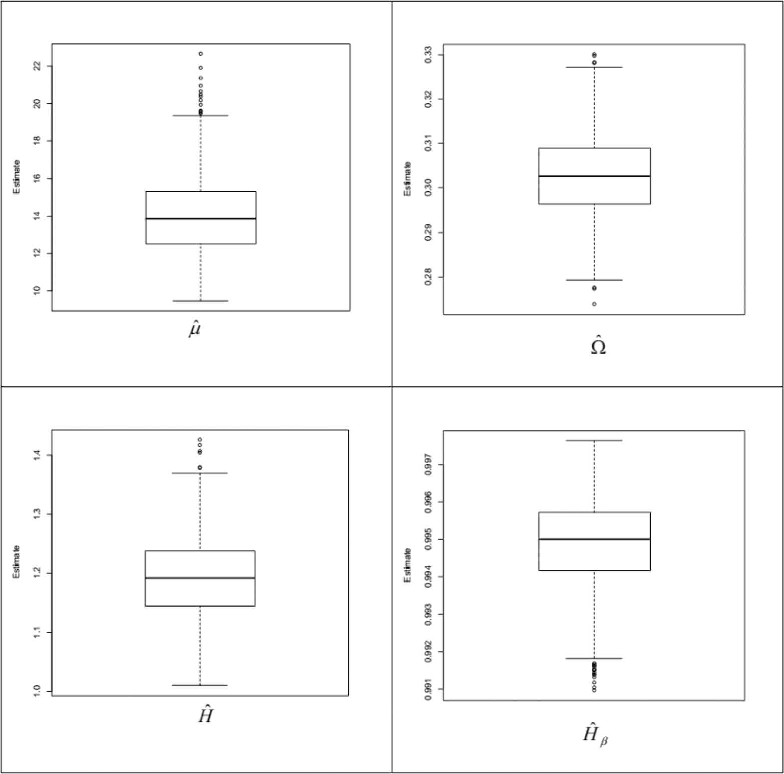
From Tables 2 and 3, we see that in most of the considered cases, the MSE of the estimation parameters decrease as n increases. The first 1000 simulations of the estimates and their biases are plotted in Figures 3 and 4.
Figure 3
Box plot of the estimates Φ^=(μ^,Ω^,H^,H^β).
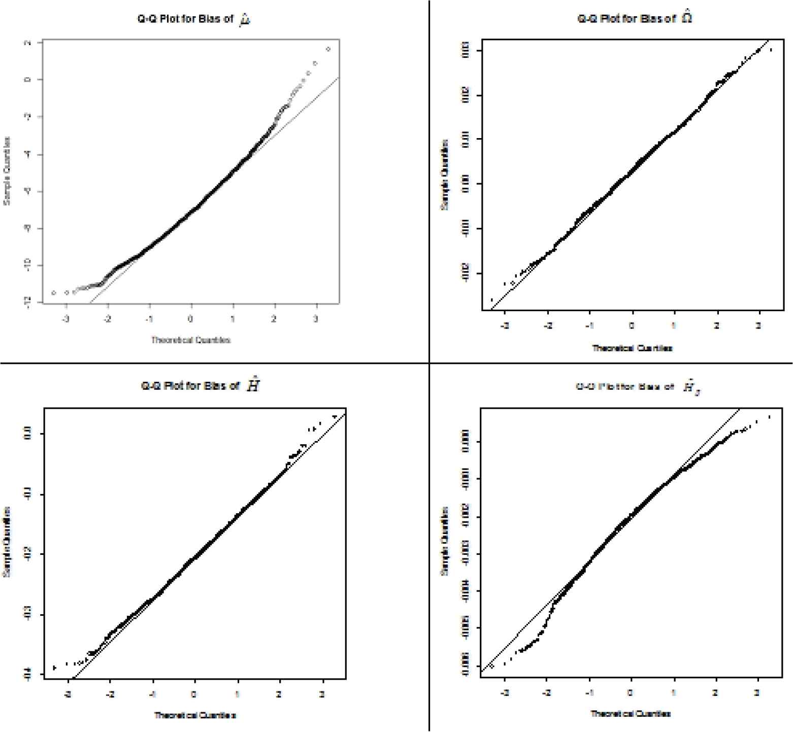
Figure 4
Q − Q plot for the bias of Φ^=(μ^,Ω^,H^,H^β).
The box plot in Figure 3 shows that among 1000 simulated estimates, there are 11 outliers for estimating μ, six outliers for estimating Ω, five outliers for estimating H and ten outliers for estimating Hβ. The probability plots in Figure 4 show that the biases of estimates, follow normal distributions that shown the data fit the GN model well, except the outliers are evident at the high and low end of the range.
Φ=(μ,Ω,H,Hβ)
n
μ̂
Ω̂
H^
H^β
25
1.66471
−0.0097242
0.1288861
0.3051938
9,0.05,1.9,0.9
50
0.83921
−0.0097206
0.1069311
0.2479989
75
0.78625
−0.0092648
0.1165099
0.0756641
100
0.49690
−0.0097457
0.0977865
0.1894217
25
6.35943
0.25078738
−0.6844654
0.1247769
21,0.3,1.4,0.997
50
5.34456
0.25220518
−0.699643
0.0948707
75
4.06696
0.23026453
−0.8001621
0.4420531
100
4.90382
0.25265919
−0.7125854
0.0991315
Table 2
Bias of the estimation of Φ^=μ^,Ω^,H^,H^β.
Φ=(μ,Ω,H,Hβ)
n
μ̂
Ω̂
H^
H^β
25
17.39353
0.000134
0.057585
2.794999
9,0.05,1.9,0.9
50
6.51417
0.000121
0.035095
2.153815
75
3.470943
8.87E-05
0.019668
0.005767
100
3.316798
0.000114
0.026113
1.46267
25
66.02313
0.063837
0.499707
0.141606
21,0.3,1.4,0.997
50
37.24665
0.063766
0.498175
0.009003
75
36.05122
0.059743
0.752393
1.621199
100
28.44723
0.064003
0.514119
0.028294
MSE: mean square errors.
Table 3
MSE of Φ^=μ^,Ω^,H^,H^β.
5. APPLICATIONS
5.1. Applications in Reliability
In next results, The application of the proposed model will be verified in the reliability theory based on three datasets. The GN distribution is compared with other usual two parameter lifetime distributions. The following lifetime distributions were considered.
5.2. Wave Height Data
The modeling of wave heights is used by mariners, as well as in coastal, ocean and naval engineering. Prevosto et al. [18], Mathiesen et al. [19] and Goda and Kobune [20] studied the heights of waves by RA distribution. In this subsection, an application of the NA distribution to this problem is described. The set of data we use are for the maximum down-crossing wave heights (Hmax D), in meters, for 23 abnormal waves, as reported by Petrova et al. ([21], p. 237). These waves were measured at the offshore platform North Alwyn in the northern part of the North Sea, about 100 miles east the Shetland Islands, during November storm in 1997.
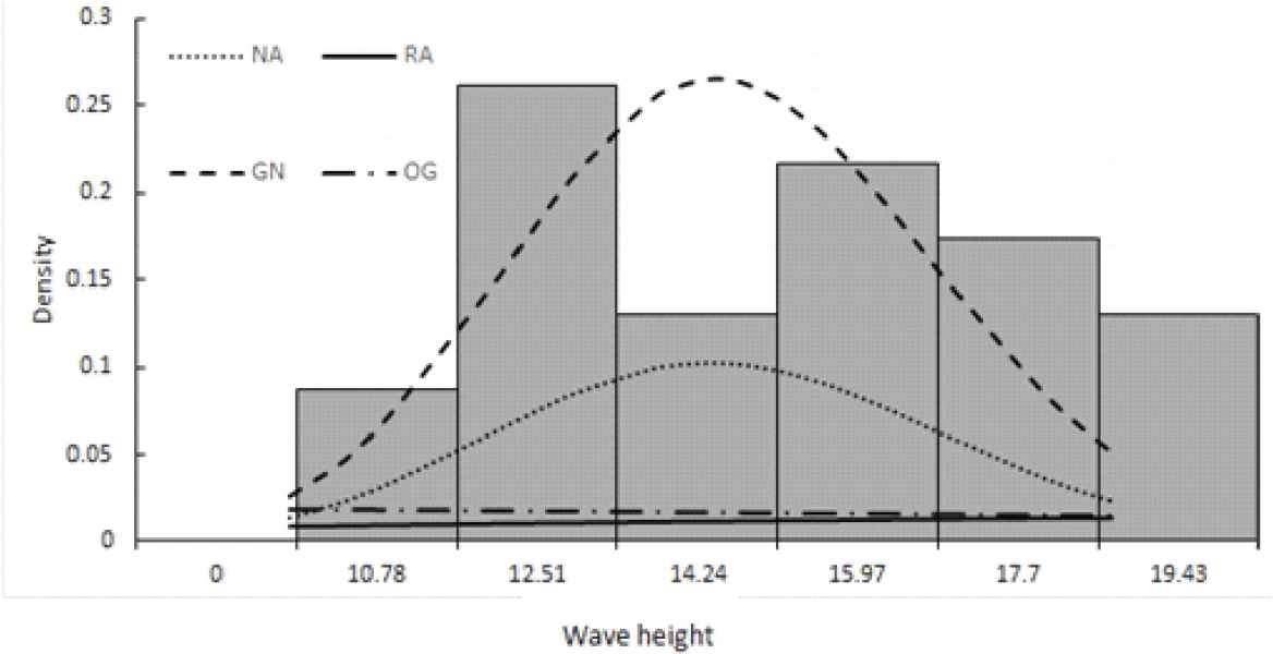
In order to compare the four distribution models, we consider the criteria like AIC (Akaike information criterion), AICC (corrected Akaike information criterion) and BIC (Bayesian information criterion). The better distribution corresponds to lesser AIC, AICc and BIC values. Table 4 indicated that the GN distribution has the lesser AIC, AICC and BIC values compared to NA distribution, OG distribution and RA distribution. Hence, we can conclude that the GN distribution leads to a better fit than other models. Further, Table 5 reports the maximum likelihood estimates of the parameters, also, 95% asymptotic confidence intervals for the parameters are provided. Moreover, Figure 5 shows empirical and fitted distribution, we see that the GN provided a better fit for this data that NA distribution, OG distribution and RA distribution.
Model
−2logL
AIC
AICc
BIC
GN
100.277
104.277
104.877
106.548
NA
140.833
144.833
145.433
147.104
OG
202.2293
204.2293
204.4198
205.3648
RA
217.1838
219.1838
219.3743
220.3193
AIC: Akaike information criterion; AICC: corrected Akaike information criterion; BIC: Bayesian information criterion; GN: Generalized Nakagami; NA: Nakagami; OG: One-sided Gaussian distribution; RA: Rayleigh distribution.
9.G.P. Patil, A.H. El-Shaarawi and W.W. Piegorsch (editors), Encyclopedia of Environmetrics, John Wiley & Sons, Chichester, England, Vol. 4, 2002.
10.A. Azzalini, Scand. J. Stat., Vol. 12, 1985, pp. 171-178.
11.I.S. Gradshteyn and I.M. Ryzhik, A. Jeffrey and D. Zwillinger (editors), Table of Integrals, Series, and Products, sixth, Academic Press, New York, NY, USA, 2000.
TY  - JOUR
AU  - Mervat Mahdy
AU  - Dina Samir
PY  - 2020
DA  - 2020/03/06
TI  - Construction, Characterization, Estimation and Performance Analysis of Selection Generalized Nakagami Distributions with Environmental Applications
JO  - Journal of Statistical Theory and Applications
SP  - 75
EP  - 90
VL  - 19
IS  - 1
SN  - 2214-1766
UR  - https://doi.org/10.2991/jsta.d.200224.003
DO  - 10.2991/jsta.d.200224.003
ID  - Mahdy2020
ER  -