
Fuzzy C-Means Clustering Using Asymmetric Loss Function
- DOI
- 10.2991/jsta.d.200302.002How to use a DOI?
- Keywords
- Fuzzy C-Means clustering; LINEX loss function
- Abstract
In this work, a fuzzy clustering algorithm is proposed based on the asymmetric loss function instead of the usual symmetric dissimilarities. Linear Exponential (LINEX) loss function is a commonly used asymmetric loss function, which is considered in this paper. We prove that the negative likelihood of an extreme value distribution is equal to LINEX loss function and clarify some of its advantages. Using such a loss function, the so-called LINEX Fuzzy C-Means algorithm is introduced. The introduced clustering method is compared with its crisp version and Fuzzy C-Means algorithms through a few real datasets as well as some simulated datasets.
- Copyright
- © 2020 The Authors. Published by Atlantis Press SARL.
- Open Access
- This is an open access article distributed under the CC BY-NC 4.0 license (http://creativecommons.org/licenses/by-nc/4.0/).
1. INTRODUCTION
Clustering is a method of creating groups of objects or clusters, in such a way that the objects in one cluster are very similar and the others are quite distinct. In hard clustering, one obtains a disjoint partitioning of the data such that, each data point belongs to exactly one of the partitions. In soft clustering, however, each data point has a certain probability (or possibility) of belonging to each of the partitions, which takes values between 0 and 1 [1]. One of the most widely used fuzzy clustering methods is the Fuzzy C-Means (FCM) algorithm, which introduced by Ruspini [2].
There are many techniques to group the observations into clusters, which use the loss functions to measure the dissimilarities between all pairs of observations such as Manhattan, Euclidean, Cosine, and Mahalanobis distances. A symmetric distance is useful for clustering when overestimating and underestimating of clusters are equally costly. That is, miss classifying object losses in two clusters have the same values. There is no common distance measure, which can be appropriate for all clustering applications. However, in some estimation problems, the use of an asymmetric loss function may be more suitable. To make our point clear, we give the following example:
Magic Gamma Telescope contains 19020 instances with 11 attributes, which use to depict high-energy gamma particles with the imaging technique in a ground-based aerial Cherenkov Gamma Telescope. It is split into two clusters, Gamma (signal), which includes 12332 data and Hadron (background) which includes 6688 data. The simple clustering accuracy is not significative for this data, because clustering a background event as the signal is worse than clustering a signal event as the background. The overestimation of a background event is preferable here. Therefore, using asymmetric dissimilarity measures helps us to classify data in the appropriate clusters to reduce the errors and risks resulting from the clustering. To present these data, we simplify the dataset artificially as follows:
Consider artificial data with one attribute and two classes that denoted by “circles” and “squares.” We define an error “e” that is the number of misclassified data and a penalized error “pe,” which is equal to “e” for the circles and “2e” for the squares. The scatterplot of 12 ordered data with respect to their values is plotted as a “Benchmark data” in Figure 1.
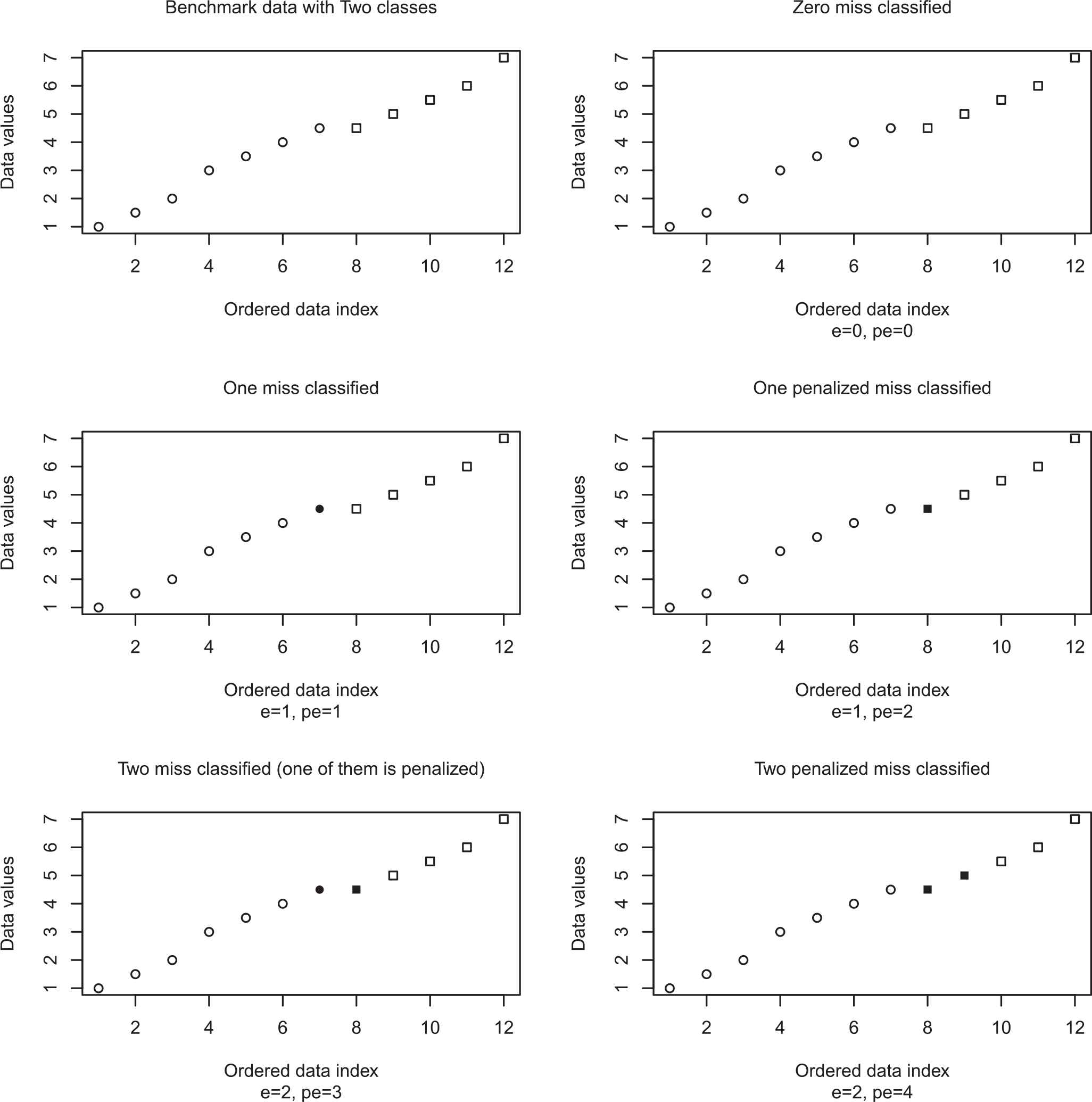
Scatterplots of 12 ordered data with one attribute and two classes that denoted by circles and squares. We use e: error, pe: penalized error. Miss classified data are bolded.
If we have no misclassified data in two clusters, both errors are zero (graph: top-right). However, when we have one misclassified data depends on it belong to which cluster the “pe” is equal to 1 for the circle and 2 for the square class (middle graphs). Note that misclassified data are bolded in the scatterplots. At the bottom of Figure 1, two cases of 2 misclassified data are plotted and two introduced errors are computed. We realize that symmetric loss function ignores such a penalty in the clustering result. Using asymmetric loss function in the estimation problem has a long history in the literature. Varian [3] and Berger [4] have considered asymmetric linear loss functions. In some estimation and prediction problems, the use of a symmetric loss function may be inappropriate. In practice, the overestimation and underestimation of the same magnitude of a parameter often have different losses, so the actual loss functions are asymmetric. Varian [3] proposed the asymmetric LINEX loss function in which, a given positive error might be more serious than a negative one of the same magnitude or vice versa [5]. Singh [6] used LINEX loss function to obtain an improved estimator for the mean in a negative exponential distribution. On the other hand, using an asymmetric loss function in clustering is used in the last decade. Soft clustering approach with Bregman divergences loss function was introduced in [7]. They proposed Bregman divergences as a dissimilarity measure for data drawn from the exponential family of distributions. Ahmadzadehgoli et al. [8] used the LINEX loss function as a dissimilarity measure in K-Means (KM) clustering. The main difference of LINEX loss function as the dissimilarity measure with respect to the introduced dissimilarity measure such as Bregman divergences in the KM clustering is the centers of clusters in the LINEX K-Means (LKM) algorithm are not the mean of their observations.
In this paper, we propose FCM clustering based on the LINEX loss function, which is called LINEX Fuzzy C-Means (LFCM). The paper is organized as follows: In Section 2, we recall the FCM algorithm. The LFCM clustering is introduced in Section 3. A characterization result and some advantages of LINEX loss function are proved and introduced in Section 4. Next, we evaluate the proposed algorithm by using some real datasets in Section 5. Section 6 dedicates to the robustness of the proposed algorithm. We conclude the paper in Section 7.
2. FUZZY C-MEANS
The FCM is a method of clustering, which allows one observation to belong to more than one cluster with a grade of membership ranging from 0 to 1. This method was introduced by Ruspini in 1970 [2], developed by Dunn in 1973 [9] and improved by Bezdek [10] in 1981. FCM has been widely used in cluster analysis, pattern recognition, and image processing. The FCM algorithm is more suited to data, which is more or less evenly distributed around the cluster centers. FCM partitions a given dataset
The FCM algorithm is shown in the following steps [10,1,11]:
Choose initial centers
Compute the membership functions
Update the cluster's center by the following expression:
Let
3. LINEX FCM CLUSTERING
Many symmetric dissimilarity measures, such as squared Euclidean, Mahalanobis, Itakura-Saito, and relative entropy, have been used for clustering. When the overestimation and the underestimation of clusters are not of the same importance, an asymmetric dissimilarity measure is more appropriate. In this case, we propose the LINEX loss function as the dissimilarity measure in the FCM clustering algorithm.
The
We want to state the LFCM algorithm, so consider the minimization equation (1), with the following
Now, we should minimize
Step 1: Fix
Step 2: Fix
The proofs of equations (3) and (4) are given in Appendices A and B, respectively. Therefore, to optimize
4. LINEX LOSS ADVANTAGES
It is well known that the best estimator of the normal distribution location parameter can be obtained under squared error loss, and the estimator under absolute error loss function is not as well as it. The converse of this statement holds for Laplace distribution [14]. This observation has been extended to some classes of distributions. One of the most important extensions is the loss function for each member of the exponential family has a one to one correspondence with a Bregman divergences loss function [7]. This is a reason that some authors prefer to work with the negative log-likelihood function of data distribution instead of the loss function. That is, they prefer to find parametrically the best loss for parameters of a certain distribution. As well as the author's knowledge, this problem is not solved for the LINEX loss function. In the following, theoretically, we characterize a class of distribution, which LINEX gives the best results for the estimation of location parameters or cluster centers.
In the first step, we investigate that, is the LINEX an element of Bregman divergences loss functions? We answer this question in the first section indirectly. However, we can prove it by the contradiction method.
Consider the one-dimensional case. Assume that the LINEX loss function is a Bregman divergence. The loss function needs to satisfy the following equation for some
Hence,
Therefore, the LINEX is not a Bregman divergences loss function.
To construct a density function,
Lemma 1.
Let
This result is interesting and important since extreme value distributions play a role similar to the normal distribution in the central limit theorem, i.e., they are convergent limits of extreme values of independent and identically distributed (iid) sequences. Therefore, the LINEX gives the best result with respect to the other loss functions in estimation or clustering as extreme values dataset.
Remark 1.
The multi-parameter separable LINEX loss function of Zellner [5] given in Section 3 has a similar property as Lemma 1 for a vector of independent Gumbel distributions with different parameters.
In addition to the mentioned properties and advantages of an asymmetric loss function in a clustering problem in the first section, we can emphasize the following points: The most and the best extensions of FCM are limited to applying on a few flexible symmetric loss functions such as Minkowski and Entropy loss functions. Bregman divergence was the only well-known class of loss function, which is contained asymmetric loss and used in fuzzy clustering. The main difference between this class with the LINEX loss, in a clustering problem, is the characterization of two different classes of distributions. On the other hand, the cluster centers in the LFCM algorithm are not a weighted mean of the data in each cluster, recall equation (4).
We continue this section with a simulation study to see the performance of the proposed clustering method with respect to the KM, FCM, and LKM clustering algorithms. We consider clustering problem of two-class datasets with two independent variables. The data proportion of each class in all datasets is equal.
Three datasets of size 200 are generated from the two-component bivariate mixture of Normal, Laplace, and Gumbel distributions with the same scale and location parameters (0, 0) and (3, 3) for each class respectively, see Figure 2. We would like to show the effect of the scale parameter,

Contour levels of bivariate density of the mixture of Normal, Laplace, and Gumbel distributions with independent components and the same proportion. The location vectors in the classes are (0, 0) and (3, 3) respectively. Both classes and variables have unit scale parameters.
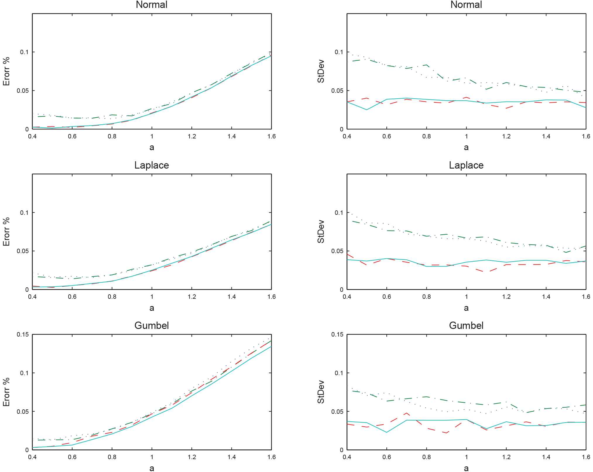
Graphs of error (miss-classified percentage) of clustered data and their StDev for the bivariate mixture of Normal, Laplace, and Gumbel distributions in Figure 1 with respect to the different scale parameters in [0.4, 1.6]. Doted, dash-dot, dashed, and solid lines present the results for KM, LKM, FCM, and LFCM algorithms, respectively.
We report the simulation result for the scale parameter in [0.4, 1.6], see Figure 3. The first observation from the graphs of this figure is the accuracy similarity of fuzzy algorithms and the similarity of non-fuzzy algorithms. That is, FCM and LFCM are better than KM and LKM in both of error percentage (left column of Figure 3) and their StDev (right column of Figure 3). In the Normal and Laplace datasets, the miss-classified percentage of FCM and LFCM are very close. However, in the Gumbel dataset LFCM is the best with the aid of Lemma 1. In overall, we can conclude that, in this experiment, LFCM is better than FCM. Also, FCM is better than LKM, which is better than KM.
In the next section, we study the preference of mentioned clustering methods through real datasets. We conclude this section with two practical remarks.
Remark 2.
The Gumbel distributions in Lemma 1 and Figure 2 are skewed to the left. If the data have a right heavy tail, the LINEX loss function is appropriate for the negative of data.
Remark 3.
In a real problem, the unknown parameter
5. EVALUATION
In this section, we employ clustering accuracy as a measure for evaluating the clustering results. Clustering accuracy is an external measure, which computes the percentage of the correctly classified data points according to the class labels [15].
We use the Normalized Variation Information (NVI) and Davies–Bouldin (DB) criteria. We compare the results with FCM and LKM clustering algorithms to check the proposed algorithm performance.
NVI is an external criterion, which is used to compare the clustering performance across original labels of datasets. If it falls in the range of
In this part, we use some real datasets, which are in the UC Irvine Machine Learning Repository [19] to verify the results of LFCM, FCM, and LKM. The datasets are listed in the following:
The Iris dataset contains 150 instances; each one consists of four features and they are grouped into three classes Setosa, Versicolour, and Virginica with 50 instances. Each class refers to a type of Iris plant.
The Wine dataset is the results of a chemical analysis of wines, which is derived from three different cultivars. It contains 178 instances; each one consists of 13 features and is grouped into three classes with 62, 69, and 47 instances.
The Seeds dataset is the examined group kernels containing 210 instances with seven features and is belonged to three varieties of wheat: Kama, Rosa, and Canadian with 70 elements.
The Haberman's Survival dataset contains 306 instances; each with three features and is grouped into two classes: the patient who is alive five years or longer and the patient died before five years.
The MAGIC Gamma Telescope contains 19020 instances; each one consists of 11 features and is grouped into two classes, Gamma (signal) with 12332 instances and Hadron (background) with 6688 instances.
Now, we want to evaluate the results on the real datasets. We run the algorithms 100 times and compute the accuracy, NVI, and DB each time for the first experiment. The results are given in Table 1. In all computations, we fix
| Dataset | Evaluation Index | FCM | ||
|---|---|---|---|---|
| LKM | LFCM | |||
| Iris | Accuracy | 0.8797 | 0.8487 | 0.8797 |
| NVI | 0.3895 | 0.4950 | 0.4005 | |
| DB | 0.4640 | 0.5390 | 0.4997 | |
| Wine | Accuracy | 0.7136 | 0.7212 | 0.6619 |
| NVI | 0.7332 | 0.7122 | 0.7690 | |
| DB | 0.4872 | 0.4871 | 0.4723 | |
| Seeds | Accuracy | 0.8744 | 0.8714 | 0.8744 |
| NVI | 0.4675 | 0.4495 | 0.4675 | |
| DB | 0.6788 | 0.8558 | 0.6788 | |
FCM, Fuzzy C-Means; LKM, LINEX K-Means; LFCM, LINEX Fuzzy C-Means; NVI, Normalized Variation Information; DB, Davies–Bouldin.
The comparison between FCM, LKM, and LFCM in terms of accuracy, NVI and DB values in real datasets. The best values are bolded.
The results in Table 1 show that the LFCM algorithm performance is not so different from the FCM for the values of the parameter
Recall the example in the first section. In the Magic Gamma Telescope dataset, underestimation of backgrounds has more penalty with respect to the signals. Therefore, calculated accuracy in Table 1 are not fair for comparing clustering algorithms. In the next experiment, we try to show the efficiency of the proposed algorithm when a penalty considered for underestimation. We assume that loss of a background classified as signal be two units and the converse be one unit. Then the loss of miss-classified data with considering a penalty, which is computed as follows:
| Dataset | Evaluation Index | FCM | LKM | LFCM |
|---|---|---|---|---|
| Haberman's survival | Accuracy | 0.5196 | 0.7164 | 0.7581 |
| NVI | 1.0000 | 0.9998 | 0.9579 | |
| DB | 0.9652 | 0.9013 | 0.9579 | |
| Penalize loss | 0.6274 | 0.4313 | 0.4151 | |
| Magic gamma telescope | Accuracy | 0.6113 | 0.6832 | 0.7015 |
| NVI | 0.9949 | 0.1230 | 0.9620 | |
| DB | 1.3770 | 0.8920 | 1.8950 | |
| Penalize loss | 0.6130 | 0.7967 | 0.5413 |
FCM, Fuzzy C-Means; LKM, LINEX K-Means; LFCM, LINEX Fuzzy C-Means; NVI, Normalized Variation Information; DB, Davies–Bouldin.
The comparison between FCM, LKM, and LFCM in terms of accuracy, NVI and DB values in real datasets with overestimation. The best values are bolded.
6. COMPLEXITY AND ROBUSTNESS
The main difference between KM and LKM is due to the center of a cluster. It is well known that, in KM algorithm, the centers of clusters are the means of clusters. However, for the LKM the centers deviate from the mean of clusters, based on the underestimating or overestimating strategy. This is the case for the FCM and LFCM. In step 3 of the FCM algorithm, the centers of clusters are recalled, which are the weighted means of the corresponding classes. We calculate the centers for the LFCM in (4), see Appendix B. By this introduction, we see that the LKM or LFCM just modified centers based on a new criterion. Therefore, the complexity of the proposed algorithm is similar to the FCM.
To show the robustness of the proposed algorithm, we consider five criteria or parameters and try to explain the behavior of the proposed algorithm through an experiment, which is classified in Table 2. The results confirm the similarity of LFCM and FCM for the convergence behavior, robustness, and sensitivity of the mentioned criteria in Table 3.
| Robustness | Experiment | Result | Conclusion |
|---|---|---|---|
| Convergence behavior | We repeat the LFCM three times for simulated and real datasets that introduced in Section 4. Based on the stopping error |
Reach to fixed points of the final centers. The recorded maximum number of iterations were obtained 18 and 47 for the simulated and real datasets. | This experiment confirms theoretical results. |
| Scalability | The convergence behaviors of the LFCM algorithm for simulated data with sizes 200, 2000, and 20000 are considered. | We have observed that the algorithm converges before iteration 40. | This confirms the computational complexity of LFCM in this range of data size. |
| Influence of the fuzziness parameter | We choose different values of |
Based on each evaluation criterion, we have a better |
We should choose an appropriate evaluation criterion before finding the best value of |
| Sensitivity to the stop condition | We choose different values of stopping error threshold |
The performance of the algorithm in some datasets has not been affected by the values of |
The range of (0.01, 0.1) for |
| Sensitivity to initialization | We run the algorithm 100 times with random seed numbers. The convergence of evaluation criteria is considered. We consider accuracy, NVI, and DB criteria. | All criteria are convergent. | LFCM is robust with respect to the initialization. |
LFCM, LINEX Fuzzy C-Means; NVI, Normalized Variation Information; DB, Davies–Bouldin.
Results of investigating five robustness criteria, experiment, result, and its conclusion for the proposed algorithm.
7. CONCLUSION
The type of distance based on loss function has an important role in the clustering analysis. When the overestimating or underestimating has the same magnitude, the symmetric loss function is a suitable one. However, when they have different significances, an asymmetric loss function should be employed. In this paper, the well-known LINEX loss function, as the asymmetric dissimilarity distance, was used to develop a new fuzzy clustering method. We stated and proved a characterization lemma to show that LFCM give an optimal result for datasets from Gumbel distribution, which is an extreme value distribution. The performance of the proposed algorithm was presented in a simulation study. Some real datasets were used to investigate the results of the LFCM and to compare with the LKM and FCM clustering algorithms. The comparisons were done based on NVI and DB criteria. The accuracy of the LFCM algorithm was good and depended on the parameter
CONFLICT OF INTEREST
Authors have no conflicts of interest to declare.
ACKNOWLEDGMENTS
The authors would like to thank the editor and the anonymous reviewers for their useful comments and suggestions that improve the manuscript, especially in Section 5. We also thank Prof. K. Shafie for his comments on the revised part of the manuscript.
APPENDIX A
The object function
To find
Put
Let
The Lagrangian of
From (A.2)
Then,
From (A.1)
Hence,
Substitute (A.4) in (A.3), we obtain
APPENDIX B
(Proof of minimizing
To prove, it is sufficient to minimize the following inner sum for fixed
To do this, we differentiate with respect to
REFERENCES
Cite this article
TY  - JOUR
AU  - Israa Abdzaid Atiyah
AU  - Adel Mohammadpour
AU  - Narges Ahmadzadehgoli
AU  - S. Mahmoud Taheri
PY  - 2020
DA  - 2020/03/09
TI  - Fuzzy C-Means Clustering Using Asymmetric Loss Function
JO  - Journal of Statistical Theory and Applications
SP  - 91
EP  - 101
VL  - 19
IS  - 1
SN  - 2214-1766
UR  - https://doi.org/10.2991/jsta.d.200302.002
DO  - 10.2991/jsta.d.200302.002
ID  - Atiyah2020
ER  -