
Robust Mixture Regression Based on the Mixture of Slash Distributions
- DOI
- 10.2991/jsta.d.200304.001How to use a DOI?
- Keywords
- EM algorithm; Normal mixture regression; Outliers; Slash distribution
- Abstract
The traditional estimation of Mixture regression models is based on the normal assumption of component errors and thus is sensitive to outliers and heavy-tailed errors. In this paper, we propose a robust Mixture regression models in which a mixture of slash distributions is assumed for the errors. Using the fact that the slash distribution can be written as a scale mixture of a normal and a latent distribution, we also estimate model parameters an expectation-maximization (EM) algorithm. The results of our simulation show that based on AIC and BIC criterion, the proposed robust regression model mixture on slash distribution dominates the robust regression based the normal and the
- Copyright
- © 2020 The Authors. Published by Atlantis Press SARL.
- Open Access
- This is an open access article distributed under the CC BY-NC 4.0 license (http://creativecommons.org/licenses/by-nc/4.0/).
1. INTRODUCTION
Mixture models are applied in such diverse areas as biology, biometrics, genetics, medicine and marketing, among others. For a brief list of application of the MRM, see Table 1. There are various features of (finite) mixture distributions that make them useful in statistical modeling. For instance, statistical models on the base of finite mixture distributions can capture various properties of real data sets such as multimodality, skewness, kurtosis and unobserved heterogeneity. For more details, see [1–5].
| Area of Application of MRM | References |
|---|---|
| Introduced by | [6] |
| Marketing | [7–9] |
| Economics | [10,11] |
| Agriculture | [12] |
| Nutrition | [13] |
| Psychometrics | [14] |
Various application of the mixture regression model (MRM).
Mixture regression models (hereafter MRM), have been widely used to investigate the relationship between variables coming from several unknown latent homogeneous groups.
The model setting for mixtures of linear regression models can be stated as follows: Let
The log-likelihood function (LLF) for observations
The computation can be further simplified based on the fact that the slash distribution can be considered as a scale mixture of normal distributions. Let
The unknown parameters in the model (2) can be estimated maximizing the LLF (3). Since the LLF (3) complicated, the maximum likelihood estimations (MLEs) are derived by maximizing (3) numerically. Among numerically methods for maximizing (3), the EM algorithm is commonly used; see [15].
The MLE
Yao et al. [21] proposed a robust estimation procedure for mixture linear regression models by assuming that the error terms follow the
Recently, researchers proposed the MRM based on skew and/or heavy tailed distributions. Lin et al. [25,4] respectively, using skew t and multivariate skew t-Normal distributions for this regression model. Song et al. [26] use the Laplace distribution. Zeller et al. [27] proposed a robust MRM based on the scale mixtures of skew-normal distributions. These authors also developed a simple EM-type algorithm to perform maximum likelihood inference of the parameters of the proposed model. In order to examine the robust aspect of this flexible model against outlying observations, some simulation studies have also been proposed. For example [28] proposed MRM using the mixture of different distributions. Dogru and Arslan [29,30] used other skew distribution for this regression model.
In recent years, attempts have been made by many researchers to propose flexible statistical models for fitting various data sets. Among the well-known distribution functions, the slash distribution, introduced by [31], provides more flexibility. See Section 2.
In this paper, we propose a robust MRM based on the slash distribution by assuming the mixture of slash distributions errors. Similar to the traditional M-estimate for linear regression (see [32]), the proposed estimate is expected to be sensitive to high leverage outliers. To overcome this problem, we also propose a modified version of the new method by fitting the new model to the data after adaptively trimming high leverage points. Compared to the TLE, the proportion of trimming of the new proposed model is data adaptive instead of a fixed value. Using a simulation study and real data application, we compare the new method to some existing methods, and demonstrate the effectiveness of the proposed method.
Therefore, the rest of this paper is organized as follows: In Section 2 the slash distribution and its properties are reviewed. In Section 3, we introduce our new robust mixture linear regression models based on the slash distribution and then develop the respective EM algorithm. In Section 4, we propose to further improve the robustness of the proposed method against high leverage outliers by adaptively trimming high leverage points. Also in this section, with simulation study, we compare the proposed method to the traditional MLE and some other robust methods by using a simulation study. Finally in Section 5, these results have been applied in real data.
The slash distribution with parameter
2. THE SLASH DISTRIBUTION
In this section, in order to more robustly estimate the mixture regression parameters, we assume that the error density function in (1) is a slash distribution with parameter
The MRM with slash distribution can be formulated in a similar way to the model defined in (2) as follows:
Note that the LLF (6) is unbounded if one of the observations
3. MAXIMUM LIKELIHOOD ESTIMATION
In this subsection, we present an EM algorithm for the ML estimation of the MRM with the slash distribution given by (5). For
If the complete data set
Based on the theory of EM algorithm, in E-step, given current estimate
Note that the above maximizer does not have explicit solutions for
Since, we can simplify the computation of M-step of the proposed EM algorithm by introducing another latent variable
In the E-step on the
Choose some initial value
E-step: On the
andwhereM-step: On the
andRepeat the E-step and the M-step until the convergence is obtained. One stopping rule that we can choose is to stop the iteration when the change of the likelihood value is smaller than
Remarke:
If we further assume that all
3.1. Initial Point in the EM Algorithm
It is well known that mixture models may provide a multimodal LLF. In this sense, the method of MLE through EM algorithm may not give maximum global solutions if the starting values are far from the real parameter values. Thus, the choice of starting values for the EM algorithm in the mixture context plays an important role in parameters estimation. In our example and simulation studies, we consider the following procedure for the slash MRM.
Partition the sample into
Compute the proportion of data points belonging to the same cluster
For each group
3.2. Evaluation of the Standard Errors from the EM-Algorithm
In this subsection, we use the results of [43] to obtain the standard errors of the estimators from the EM-algorithm. For evaluation of the standard errors, one can also see [44]. Let
Taking the conditional expectation of
Moving now to the computation of
The standard errors of the MLEs of the EM-algorithm are the inverse of square root of the diagonal elements of the
4. SIMULATION STUDY
To assess the finite sample performance of the proposed model and the estimation procedure, we conducted an simulation study. In the EM algorithm, it is well khnown that label switching is always an issue when evaluating different estimation methods in mixture models, and there are no widely accepted labeling standards. In this simulation study, we choose the labels by minimizing the distance to the true parameter values. However, more research on choosing labels is needed (see [45]). Also, we considered equal variance for all components. The reason is that, if the variances are not same, the LLF (7) is unbounded and tends to infinity if one observation lies exactly on one component line and the corresponding variance vanishes, which makes the simulation very unstable.
4.1. Evaluate Robustness of the MRM
We use the method that proposed by [21] for evaluating robustness of the MRM. They proposed a trimmed version of the new method by fitting the new model to the data after adaptively trimming high leverage points. In addition, unlike
Suppose that
Case (I):
Case (II):
Case (III):
Case (IV):
Case (V):
Case (VI):
Case (I) is often used to evaluate the efficiency of different estimation methods compared to the traditional MLE when the error is normally distributed and there is no outliers. For Case (II), the estimation methods proposed in this paper will provide the MLE of unknown parameters, which, as in the first case, would serve as a baseline to evaluate the performance of other estimation procedures. Cases (III) and (IV) are heavy tailed distribution and are often used in the literature to mimic the outlier situations. Case (V) would produce 5% data likely to be low leverage outliers, and in Case (VI), 5% of the observations are replicated serving as the high leverage outliers, which will be used to check the robustness of estimation procedures against the high leverage outliers.
Five estimation methods were compared in the simulation study: (1) the maximum likelihood method based on the normality assumption (MLE); (2) the TLE proposed by [18]; (3) the robust modified EM algorithm based on bisquare (Bisquare) proposed by [19]; (4) the proposed robust EM mixture regression method based on the slash distribution (Mixregs); (5) the trimmed mixture regression method based on the slash distribution (Mixregs-MCD), with MCD trimming method. In the iterative numerical methods, the iteration is terminated when the change in the likelihood function is less than
Tables 2–5 report the mean squared errors (MSE) and the absolute bias (Bias) of the parameter estimates for each estimation method for sample sizes
| True | MLE | TLE | Bisquare | Mixregt | Mixregt-MCD | Mixregs | Mixregs-MCD |
|---|---|---|---|---|---|---|---|
| Case (I): |
|||||||
| 0.0035(0.4785) | 0.0109(0.6015) | 0.0040(0.4875) | 0.0032(0.4561) | 0.0071(0.5167) | 0.0001(0.3494) | 0.0056(0.3770) | |
| 0.1528(0.5638) | 0.8904(1.5952) | 0.4678(0.9193) | 0.2377(0.6354) | 0.2862(0.7588) | 0.0495(0.3492) | 0.0722(0.4207) | |
| 0.1366(0.5285) | 0.8904(1.5965) | 0.4586(0.8733) | 0.2217(0.6059) | 0.2696(0.7172) | 0.0393(0.3625) | 0.0612(0.4490) | |
| 0.0006(0.0869) | 0.0053(0.2304) | 0.0038(0.1296) | 0.0019(0.0981) | 0.0059(0.1269) | 0.0012(0.0455) | 0.0024(0.0544) | |
| 0.0058(0.0627) | 0.0212(0.1404) | 0.0277(0.0879) | 0.0084(0.0702) | 0.0068(0.0985) | 0.0074(0.0472) | 0.0027(0.0661) | |
| 0.0160(0.0680) | 0.0275(0.1278) | 0.0432(0.0906) | 0.0212(0.0663) | 0.0246(0.0933) | 0.0013(0.0483) | 0.0007(0.0654) | |
| 0.0326(0.0120) | 0.1413(0.0374) | 0.0891(0.0259) | 0.0510(0.0149) | 0.0626(0.0182) | 0.0003(0.0130) | 0.0068(0.0151) | |
| Case (II): |
|||||||
| 0.0592(52.9240) | 0.0066(1.5574) | 0.0065(1.5919) | 0.0178(3.9062) | 0.0531(4.1787) | 0.0160(0.7033) | 0.0200(0.8057) | |
| 0.5294(65.3548) | 0.7148(1.9506) | 0.5117(1.6059) | 0.3411(4.5422) | 0.3415(4.9709) | 0.0460(0.6372) | 0.0646(0.8130) | |
| 0.2843(39.1912) | 0.7195(1.8359) | 0.5054(1.6077) | 0.4040(4.0941) | 0.3734(4.7012) | 0.0409(0.6399) | 0.0537(0.8949) | |
| 0.0018(38.2963) | 0.0035(0.8519) | 0.0112(0.7225) | 0.0548(2.7391) | 0.0200(2.6460) | 0.0020(0.0799) | 0.0028(0.0895) | |
| 1.0935(36.3988) | 0.0835(0.6123) | 0.1200(0.6647) | 0.2309(3.0690) | 0.2967(4.3152) | 0.0073(0.0898) | 0.0082(0.1115) | |
| 1.2521(41.2024) | 0.0899(0.5964) | 0.1553(0.5842) | 0.2122(2.8183) | 0.2575(3.6373) | 0.0023(0.0891) | 0.0042(0.1058) | |
| 0.1820(0.1555) | 0.1717(0.0547) | 0.1528(0.0570) | 0.1505(0.0643) | 0.1592(0.0695) | 0.0122(0.0278) | 0.0122(0.0288) | |
| Case (III): |
|||||||
| 11.6090(501705.6719) | 0.1484(36.6703) | 0.0082(2.7508) | 0.0009(9.2711) | 0.0010(10.8682) | 0.0161(1.6247) | 0.0444(1.7095) | |
| 21.7989(49070.7569) | 0.1158(37.1632) | 0.5407(3.0793) | 0.4597(12.4083) | 0.2960(22.9286) | 0.0536(1.6220) | 0.0279(2.0650) | |
| 44.2708(1982026.0620) | 0.0477(19.2282) | 0.5466(2.7890) | 0.3747(17.2967) | 0.3317(20.0879) | 0.0122(1.9936) | 0.0154(2.3890) | |
| 6.5844(1410067.1062) | 0.0457(13.4585) | 0.0426(8.4725) | 0.0329(13.4541) | 0.0239(14.6770) | 0.0048(0.1757) | 0.0021(0.1658) | |
| 48.3717(2540865.2077) | 0.5829(15.6338) | 0.1778(2.0443) | 0.4748(13.1418) | 0.5896(13.8616) | 0.0002(0.1785) | 0.0071(0.2151) | |
| 46.2134(713106.5159) | 0.6152(14.6803) | 0.2375(22.8824) | 0.4430(13.5257) | 0.4694(18.4484) | 0.0063(0.1780) | 0.0109(0.2317) | |
| 0.2414(0.2483) | 0.1746(0.1025) | 0.1844(0.0760) | 0.1769(0.0677) | 0.1829(0.0724) | 0.0193(0.0436) | 0.0226(0.0443) | |
| Case (IV): |
|||||||
| 0.0097(0.7824) | 0.0100(0.5476) | 0.0222(0.4867) | 0.0052(0.4622) | 0.0059(0.5169) | 0.0061(0.2894) | 0.0090(0.3205) | |
| 0.1221(0.8182) | 0.6228(1.1672) | 0.4430(0.9152) | 0.1946(0.6037) | 0.2138(0.6899) | 0.0309(0.2877) | 0.0716(0.4048) | |
| 0.1172(0.7817) | 0.6214(1.1486) | 0.4314(0.8522) | 0.1882(0.5904) | 0.2190(0.7188) | 0.0450(0.2821) | 0.0514(0.4334) | |
| 0.0009(0.1970) | 0.0033(0.1314) | 0.0020(0.1105) | 0.0018(0.0652) | 0.0013(0.0824) | 0.0009(0.0217) | 0.0005(0.0353) | |
| 0.0229(0.1755) | 0.0182(0.1083) | 0.0241(0.0728) | 0.0093(0.0687) | 0.0149(0.0932) | 0.0012(0.0243) | 0.0036(0.0426) | |
| 0.0413(0.1677) | 0.0269(0.0955) | 0.0457(0.0788) | 0.0207(0.0669) | 0.0242(0.0956) | 0.0018(0.0246) | 0.0070(0.0452) | |
| 0.0355 (0.0181) | 0.0953(0.0269) | 0.0872(0.0249) | 0.0450(0.0129) | 0.0530(0.0156) | 0.0086(0.0138) | 0.0112(0.0147) | |
| Case (V): |
|||||||
| 0.0239(5.1865) | 0.0070(0.6854) | 0.0129(0.6047) | 0.0077(1.1336) | 0.0053(1.2544) | 0.0000(0.2890) | 0.0009(0.3453) | |
| 0.1788(4.8738) | 0.7779(1.4818) | 0.4566(1.0430) | 0.2930(1.4110) | 0.3190(1.6596) | 0.0299(0.3321) | 0.0526(0.4502) | |
| 0.0983(5.5528) | 0.7600(1.3980) | 0.4632(0.9917) | 0.2787(1.3798) | 0.3233(1.7069) | 0.0445(0.4024) | 0.0408(0.4929) | |
| 0.0175(4.8827) | 0.0012(0.2373) | 0.0053(0.1499) | 0.0052(0.4807) | 0.0023(0.703) | 0.0115(0.0469) | 0.0114(0.0428) | |
| 0.2626(3.9198) | 0.0240(0.1881) | 0.0415(0.1316) | 0.0266(0.4103) | 0.0515(0.7089) | 0.0003(0.0413) | 0.0002(0.0594) | |
| 0.3090(3.8525) | 0.0373(0.1679) | 0.0492(0.1490) | 0.0639(0.5072) | 0.084(0.7683) | 0.0054(0.0403) | 0.0046(0.0579) | |
| 0.1009(0.0886) | 0.1257(0.0344) | 0.0994(0.0308) | 0.0749(0.0276) | 0.0908(0.0343) | 0.0037(0.0124) | 0.0003(0.0158) | |
| Case (VI): |
|||||||
| 0.0763(5.3771) | 0.0128(0.7567) | 0.0438(1.0701) | 0.1006(4.1444) | 0.0019(0.5139) | 0.0423(0.8197) | 0.0046(0.3005) | |
| 1.4844(6.1813) | 0.4397(1.3832) | 0.0892(1.4288) | 1.4920(4.6566) | 0.2778(0.7660) | 0.5649(1.2906) | 0.0066(0.3703) | |
| 1.5091(6.2501) | 0.4477(1.3542) | 0.1050(1.4845) | 1.4746(4.6102) | 0.2815(0.7487) | 0.5472(1.2253) | 0.0150(0.3632) | |
| 0.0024(0.0508) | 0.0039(0.1774) | 0.0029(0.0805) | 0.0048(0.0568) | 0.0037(0.1261) | 0.0005(0.0425) | 0.0013(0.0449) | |
| 0.2027(0.1196) | 0.0046(0.1412) | 0.0082(0.0781) | 0.1244(0.0913) | 0.0303(0.1008) | 0.0701(0.0583) | 0.0003(0.0446) | |
| 0.2099(0.1244) | 0.0050(0.1365) | 0.0030(0.0812) | 0.1338(0.0964) | 0.0237(0.1078) | 0.0677(0.0586) | 0.0004(0.0460) | |
| 0.0886(0.0102) | 0.0930(0.0247) | 0.0461(0.0193) | 0.0738(0.0089) | 0.0709(0.0204) | 0.0364(0.0129) | 0.0048(0.0123) | |
MSE, mean squared error; MLE, maximum likelihood estimations; TLE, trimmed likelihood estimator.
Bias and MSE (in parentheses) of point estimates for
| True | MLE | TLE | Bisquare | Mixregt | Mixregt-MCD | Mixregs | Mixregs-MCD |
|---|---|---|---|---|---|---|---|
| Case (I): |
|||||||
| 0.0097(0.1228) | 0.0020(0.1002) | 0.0006(0.1349) | 0.0030(0.1340) | 0.0008(0.1554) | 0.0064(0.1342) | 0.0054(0.1496) | |
| 0.0149(0.1251) | 0.0735(0.1139) | 0.0240(0.1675) | 0.0405(0.1513) | 0.0546(0.1995) | 0.0019(0.1312) | 0.0007(0.1611) | |
| 0.0030(0.1298) | 0.0747(0.1147) | 0.0328(0.1659) | 0.0392(0.1501) | 0.0580(0.1954) | 0.0044(0.1327) | 0.0098(0.1648) | |
| 0.0009(0.0188) | 0.0026(0.0168) | 0.0000(0.0210) | 0.0015(0.0218) | 0.0029(0.0255) | 0.0020(0.0204) | 0.0019(0.0218) | |
| 0.0019(0.0195) | 0.0275(0.0173) | 0.0025(0.0219) | 0.0096(0.0209) | 0.0107(0.0261) | 0.0039(0.0207) | 0.0028(0.0256) | |
| 0.0008(0.0197) | 0.0294(0.0165) | 0.0061(0.0218) | 0.0072(0.0202) | 0.0090(0.0255) | 0.0069(0.0202) | 0.0051(0.0245) | |
| 0.0006(0.0061) | 0.0523(0.0096) | 0.0025(0.0113) | 0.0117(0.0049) | 0.0157(0.0058) | 0.0042(0.0064) | 0.0026(0.0072) | |
| Case (II): |
|||||||
| 0.0883(67.0279) | 0.0005(0.9510) | 0.0018(0.9885) | 0.0182(2.1725) | 0.0104(2.5396) | 0.0008(0.6941) | 0.0049(0.6992) | |
| 0.8606(72.2127) | 0.5882(1.2027) | 0.3194(0.9784) | 0.1967(4.4901) | 0.1811(4.3832) | 0.0462(0.6795) | 0.0424(0.7862) | |
| 0.8628(49.1993) | 0.5832(1.1459) | 0.2903(0.9782) | 0.1583(3.2396) | 0.2100(3.1637) | 0.0339(0.6743) | 0.0489(0.7677) | |
| 0.1339(84.6754) | 0.0034 (0.3623) | 0.0034 (0.3351) | 0.0096 (1.5744) | 0.0138 (1.4106) | 0.0043(0.0629) | 0.0049(0.0883) | |
| 1.7241(64.2070) | 0.0364(0.1853) | 0.0829(0.2552) | 0.0985(1.1663) | 0.1289(1.2812) | 0.0052(0.0665) | 0.0054(0.1086) | |
| 1.6774(64.7592) | 0.0491(0.2135) | 0.0832(0.2432) | 0.1126(1.2056) | 0.1139(1.1414) | 0.0057(0.0688) | 0.0010(0.1151) | |
| 0.1798(0.1945) | 0.1198(0.0328) | 0.0988(0.0351) | 0.0795(0.0355) | 0.0924(0.0421) | 0.0075(0.0260) | 0.0113(0.0288) | |
| Case (III): |
|||||||
| 10.2255(502197.693) | 0.0724(7.9262) | 0.0025(1.6847) | 0.0193(2.6750) | 0.0042(2.7491) | 0.0165(0.8272) | 0.0064(0.9149) | |
| 53.9287(473663.046) | 0.2454(6.7949) | 0.4377(1.7240) | 0.5182(4.3426) | 0.5384(3.8060) | 0.0625(0.8331) | 0.0764(0.9773) | |
| 57.7344(604387.717) | 0.1955(6.1361) | 0.4510(1.7334) | 0.5412(3.3579) | 0.5114(3.6211) | 0.0624(0.8387) | 0.0637(0.9625) | |
| 13.9702(2522395.636) | 0.0047(7.0569) | 0.0081(0.7474) | 0.0597(3.4518) | 0.0420(5.3667) | 0.0005(0.0544) | 0.0047(0.0560) | |
| 92.9882(2734642.730) | 0.3511(5.3462) | 0.0773(0.5873) | 0.1203(3.2147) | 0.1104(2.5059) | 0.0136(0.0621) | 0.0165(0.0712) | |
| 81.6340(2400307.367) | 0.3780(5.6155) | 0.0908(0.5098) | 0.1038(1.3682) | 0.2075(6.1631) | 0.0122(0.0628) | 0.0148(0.0722) | |
| 0.2405(0.277) | 0.1350(0.0961) | 0.1455(0.0543) | 0.1159(0.0377) | 0.1235(0.0416) | 0.0090(0.0336) | 0.0141(0.0363) | |
| Case (IV): |
|||||||
| 0.0073(0.2388) | 0.0011(0.3148) | 0.0020(0.2660) | 0.0020(0.1306) | 0.0022(0.1452) | 0.0059(0.0958) | 0.0048(0.1045) | |
| 0.0219(0.2414) | 0.3869(0.6129) | 0.1957(0.3853) | 0.0382(0.1385) | 0.0507(0.1716) | 0.0268(0.1197) | 0.0328(0.1484) | |
| 0.0268(0.2044) | 0.4095(0.6287) | 0.1973(0.3881) | 0.0406(0.1330) | 0.0475(0.1663) | 0.0363(0.1166) | 0.0429(0.1409) | |
| 0.0027(0.0847) | 0.0033(0.0484) | 0.0010 (0.0401) | 0.0006(0.0147) | 0.0002(0.0177) | 0.0020(0.0127) | 0.0022(0.0133) | |
| 0.0219(0.0663) | 0.0046(0.0271) | 0.0202(0.0264) | 0.0066(0.0129) | 0.0065(0.0155) | 0.0018(0.0125) | 0.0017(0.0161) | |
| 0.0212(0.0428) | 0.0065(0.0274) | 0.0228(0.0256) | 0.0091(0.0139) | 0.0111(0.0173) | 0.0026(0.0115) | 0.0029(0.0158) | |
| 0.0096(0.0063) | 0.0425(0.0111) | 0.0461(0.0122) | 0.0123(0.0043) | 0.0144(0.0048) | 0.0078(0.0069) | 0.0091(0.0081) | |
| Case (V): |
|||||||
| 0.0363(5.8679) | 0.0107(0.4219) | 0.0034(0.2510) | 0.0023(0.3526) | 0.0008(0.3908) | 0.0018(0.2013) | 0.0027(0.2141) | |
| 0.0887(4.9647) | 0.6043(0.9888) | 0.1826(0.4323) | 0.0754(0.4468) | 0.0709(0.5583) | 0.0050(0.1991) | 0.0102(0.2473) | |
| 0.0461(4.9456) | 0.6089(0.9898) | 0.1928(0.4286) | 0.0797(0.4676) | 0.0964(0.5888) | 0.0077(0.2032) | 0.0096(0.2427) | |
| 0.0404(7.0121) | 0.0056(0.1193) | 0.0022(0.0542) | 0.0041(0.1568) | 0.0008(0.2250) | 0.0016(0.0243) | 0.0023(0.0256) | |
| 0.3090(4.3915) | 0.0108(0.0553) | 0.0165(0.0387) | 0.0125(0.1123) | 0.0222(0.1786) | 0.0079(0.0240) | 0.0078(0.0301) | |
| 0.2940(4.3170) | 0.0051(0.0524) | 0.0136(0.0407) | 0.0091(0.1268) | 0.0174(0.3255) | 0.0062(0.0236) | 0.0062(0.0283) | |
| 0.0871(0.0992) | 0.0781(0.0196) | 0.0460(0.0141) | 0.0203(0.0095) | 0.0238(0.0109) | 0.0049(0.0090) | 0.0040(0.0103) | |
| Case (VI): |
|||||||
| 0.1116(3.9889) | 0.0143(0.5237) | 0.0455(0.7972) | 0.1189(2.8301) | 0.0090(0.1585) | 0.0655(0.6801) | 0.0082(0.1237) | |
| 1.4606(4.5974) | 0.1432(0.8990) | 0.3537(1.0996) | 1.4982(3.6290) | 0.0629(0.2004) | 0.7505(1.3577) | 0.0019(0.1302) | |
| 1.5307(4.8079) | 0.1652(0.8693) | 0.3766(1.1550) | 1.4945(3.6208) | 0.0549(0.1984) | 0.7475(1.3744) | 0.0050(0.1253) | |
| 0.0104(0.0262) | 0.0130(0.0896) | 0.0003(0.0426) | 0.0105(0.0612) | 0.0025(0.0269) | 0.0061(0.0196) | 0.0003(0.0192) | |
| 0.2252(0.0901) | 0.0131(0.0849) | 0.0181(0.0337) | 0.1373(0.0726) | 0.0071(0.0265) | 0.1090(0.0441) | 0.0010(0.0199) | |
| 0.2277(0.0932) | 0.0204(0.0884) | 0.0221(0.0371) | 0.1352(0.0745) | 0.0111(0.0267) | 0.1040(0.0409) | 0.0018(0.0207) | |
| 0.0890(0.0092) | 0.0353(0.0107) | 0.0006(0.0087) | 0.0762(0.0076) | 0.0169(0.0062) | 0.0624(0.0171) | 0.0006(0.0061) | |
MSE, mean squared error; MLE, maximum likelihood estimations; TLE, trimmed likelihood estimator.
Bias and MSE (in parentheses) of point estimates for
| True | MLE | TLE | Bisquare | Mixregt | Mixregt-MCD | Mixregs | Mixregs-MCD |
|---|---|---|---|---|---|---|---|
| Case (I): |
|||||||
| 0.0003(0.0451) | 0.0001(0.0364) | 0.0001(0.0504) | 0.0031(0.0443) | 0.0029(0.0474) | 0.0035(0.0483) | 0.0033(0.0517) | |
| 0.0039(0.0441) | 0.0407(0.0376) | 0.0024(0.0547) | 0.0051(0.0418) | 0.0076(0.0493) | 0.0037(0.0461) | 0.0065(0.0581) | |
| 0.0084(0.0451) | 0.0417(0.0374) | 0.0010(0.0559) | 0.0065(0.0415) | 0.0092(0.0497) | 0.0084(0.0470) | 0.0090(0.0576) | |
| 0.0015(0.0093) | 0.0000(0.0075) | 0.0014(0.0100) | 0.0005(0.0092) | 0.0007(0.0094) | 0.0029(0.0086) | 0.0030(0.0091) | |
| 0.0006(0.0093) | 0.0305(0.0086) | 0.0018(0.0101) | 0.0044(0.0089) | 0.0059(0.0104) | 0.0012(0.0091) | 0.0027(0.0108) | |
| 0.0015(0.0089) | 0.0299(0.0084) | 0.0001(0.0099) | 0.0021(0.0090) | 0.0038(0.0105) | 0.0003(0.0094) | 0.0002(0.0112) | |
| 0.0002(0.0026) | 0.0581(0.0071) | 0.0000(0.0038) | 0.0031(0.0022) | 0.0043(0.0024) | 0.0020(0.0028) | 0.0021(0.0032) | |
| Case (II): |
|||||||
| 0.2238(129.3761) | 0.0066(0.4795) | 0.0129(0.4322) | 0.0154(0.5663) | 0.0154(0.9366) | 0.0035(0.2805) | 0.0050(0.3098) | |
| 1.6322(103.4913) | 0.4177(0.6341) | 0.0836(0.4221) | 0.0852(0.6943) | 0.0707(1.6737) | 0.0240(0.3173) | 0.0348(0.3931) | |
| 1.7944(107.1121) | 0.4148(0.6227) | 0.0760(0.4140) | 0.0886(0.7964) | 0.0803(1.2111) | 0.0225(0.3114) | 0.0294(0.3955) | |
| 0.0987(147.1717) | 0.0004(0.1309) | 0.0026(0.0980) | 0.0058(0.4486) | 0.0083(0.3612) | 0.0028(0.0209) | 0.0008(0.0341) | |
| 2.4287(134.7825) | 0.0230(0.0640) | 0.0429(0.0570) | 0.0314(0.4694) | 0.0411(0.3362) | 0.0044(0.0292) | 0.0009(0.0499) | |
| 2.4348(119.5413) | 0.0221(0.0638) | 0.0472(0.0604) | 0.0321(0.2403) | 0.0400(0.5037) | 0.0046(0.0279) | 0.0027(0.0494) | |
| 0.1839 (0.2251) | 0.0767(0.0158) | 0.0540(0.0144) | 0.0320(0.0117) | 0.0397(0.0158) | 0.0063(0.0140) | 0.0121(0.0182) | |
| Case (III): |
|||||||
| 25.0509(1.909716e+06) | 0.0184(4.7935) | 0.0115(0.7171) | 0.0164(0.5915) | 0.0047(0.6980) | 0.0102(0.2730) | 0.0078(0.2782) | |
| 131.7579(2.203641e+06) | 0.1625(3.3181) | 0.2768(0.9563) | 0.3669(1.1273) | 0.3668(1.4800) | 0.0552(0.3230) | 0.0797(0.4144) | |
| 101.4703(1.798630e+06) | 0.1445(3.4201) | 0.2997(0.9783) | 0.3612(1.2457) | 0.3758(1.2865) | 0.0528(0.3290) | 0.0604(0.3898) | |
| 1584.5368(1.254946e+10) | 0.0478(3.7613) | 0.0008(0.3362) | 0.0060(0.2418) | 0.0056(0.2008) | 0.0024(0.0213) | 0.0025(0.0230) | |
| 1150.8596(5.003399e+09) | 0.1862(2.2135) | 0.0526(0.2070) | 0.0363(0.2245) | 0.0363(0.4318) | 0.0028(0.0241) | 0.0040(0.0292) | |
| 3101.5797(4.430502e+10) | 0.1874(2.2794) | 0.0424(0.2205) | 0.0307(0.2821) | 0.0440(0.5097) | 0.0000(0.0248) | 0.0016(0.0303) | |
| 0.2413(2.912000e-01) | 0.0894(0.0751) | 0.1199(0.0353) | 0.0654(0.0199) | 0.0706(0.0218) | 0.0120(0.0179) | 0.0164(0.0211) | |
| Case (IV): |
|||||||
| 0.0024(0.0480) | 0.0028(0.1411) | 0.0029(0.0749) | 0.0008(0.0313) | 0.0005(0.0339) | 0.0000(0.0223) | 0.0006(0.0346) | |
| 0.0055(0.0481) | 0.2040(0.2414) | 0.0453(0.0997) | 0.0060(0.0302) | 0.0056(0.0356) | 0.0107(0.0249) | 0.0137(0.0423) | |
| 0.0023(0.0551) | 0.2173(0.2563) | 0.0456(0.0974) | 0.0073(0.0293) | 0.0092(0.0346) | 0.0146(0.0250) | 0.0186(0.0441) | |
| 0.0017(0.0485) | 0.0029(0.0154) | 0.0011(0.0078) | 0.0007(0.0053) | 0.0008(0.0055) | 0.0000(0.0060) | 0.0001(0.0062) | |
| 0.0115(0.0077) | 0.0049(0.0092) | 0.0114(0.0070) | 0.0019(0.0050) | 0.0026(0.0059) | 0.0034(0.0058) | 0.0045(0.0068) | |
| 0.0148(0.0200) | 0.0014(0.0098) | 0.0123(0.0072) | 0.0032(0.0053) | 0.0037(0.0061) | 0.0033(0.0061) | 0.0041(0.0070) | |
| 0.0036(0.0023) | 0.0207(0.0046) | 0.0265(0.0036) | 0.0057(0.0020) | 0.0063(0.0021) | 0.0054(0.0028) | 0.0066(0.0032) | |
| Case (V): |
|||||||
| 0.0627(5.4191) | 0.0003(0.2256) | 0.0010(0.0908) | 0.0002(0.0786) | 0.0005(0.0754) | 0.0042(0.0726) | 0.0005(0.0767) | |
| 0.0103(4.9720) | 0.4269(0.5704) | 0.0495(0.1354) | 0.0100(0.0845) | 0.0129(0.0931) | 0.0006(0.0674) | 0.0060(0.0811) | |
| 0.0643(4.7922) | 0.4246(0.5647) | 0.0499(0.1379) | 0.0075(0.0821) | 0.0086(0.0900) | 0.0098(0.0679) | 0.0128(0.0859) | |
| 0.0544(6.3131) | 0.0029(0.0504) | 0.0015(0.0136) | 0.0014(0.0117) | 0.0010(0.0129) | 0.0001(0.0102) | 0.0000(0.0108) | |
| 0.2140(3.8070) | 0.0014(0.0195) | 0.0086(0.0135) | 0.0008(0.0112) | 0.0009(0.0144) | 0.0017(0.0108) | 0.0018(0.0129) | |
| 0.2437(4.0257) | 0.0015(0.0192) | 0.0080(0.0137) | 0.0019(0.0111) | 0.0019(0.0147) | 0.0011(0.0103) | 0.0030(0.0125) | |
| 0.0574(0.0849) | 0.0365(0.0084) | 0.0229(0.0063) | 0.0013(0.0027) | 0.0022(0.0031) | 0.0014(0.0038) | 0.0007(0.0044) | |
| Case (VI): |
|||||||
| 0.1759(2.6488) | 0.0012(0.2241) | 0.0576(0.4823) | 0.1315(1.8995) | 0.0015(0.0496) | 0.0717(0.4401) | 0.0015(0.0442) | |
| 1.4949(3.5135) | 0.0875(0.3978) | 0.3566(0.7782) | 1.5023(3.0228) | 0.0089(0.0493) | 0.6859(1.1268) | 0.0033(0.0466) | |
| 1.4925(3.5030) | 0.0779(0.4179) | 0.3686(0.8232) | 1.4895(2.9826) | 0.0040(0.0522) | 0.6703(1.0896) | 0.0048(0.0478) | |
| 0.0080(0.0145) | 0.0037(0.0366) | 0.0006(0.0105) | 0.0072(0.0271) | 0.0011(0.0096) | 0.0013(0.0098) | 0.0015(0.0099) | |
| 0.2441(0.0798) | 0.0172(0.0465) | 0.0259(0.0129) | 0.1376(0.0679) | 0.0048(0.0104) | 0.1002(0.0312) | 0.0002(0.0091) | |
| 0.2445(0.0800) | 0.0188(0.0460) | 0.0266(0.0126) | 0.1421(0.0652) | 0.0004(0.0104) | 0.1035(0.0314) | 0.0031(0.0092) | |
| 0.0954(0.0098) | 0.0070(0.0041) | 0.0138(0.0044) | 0.0836(0.0080) | 0.0042(0.0025) | 0.0561(0.0159) | 0.0008(0.0026) | |
MSE, mean squared error; MLE, maximum likelihood estimations; TLE, trimmed likelihood estimator.
Bias and MSE (in parentheses) of point estimates for
| True | MLE | TLE | Bisquare | Mixregt | Mixregt-MCD | Mixregs | Mixregs-MCD |
|---|---|---|---|---|---|---|---|
| Case (I): |
|||||||
| 0.0001(0.0123) | 0.0001(0.0115) | 0.0000(0.0019) | 0.0030(0.0098) | 0.0028(0.0113) | 0.0010(0.0203) | 0.0011(0.0213) | |
| 0.0012(0.0131) | 0.0290(0.0191) | 0.0013(0.0023) | 0.0017(0.0083) | 0.0037(0.0094) | 0.0031(0.0185) | 0.0058(0.0225) | |
| 0.0086(0.0124) | 0.0312(0.0189) | 0.0008(0.0028) | 0.0034(0.0070) | 0.0039(0.0199) | 0.0034(0.0191) | 0.0049(0.0226) | |
| 0.0019(0.0012) | 0.0000(0.0011) | 0.0012(0.0011) | 0.0002(0.0013) | 0.0000(0.0021) | 0.0015(0.0043) | 0.0032(0.0044) | |
| 0.0002(0.0011) | 0.0313(0.0009) | 0.0009(0.0013) | 0.0011(0.0010) | 0.0023(0.0056) | 0.0003(0.0043) | 0.0008(0.0051) | |
| 0.0016(0.0065) | 0.0181(0.0011) | 0.0001(0.0008) | 0.0013(0.0011) | 0.0016(0.0059) | 0.0005(0.0044) | 0.0003(0.0051) | |
| 0.0001(0.0011) | 0.0652(0.0020) | 0.0000(0.0011) | 0.0024(0.0009) | 0.0023(0.0012) | 0.0011(0.0012) | 0.0017(0.0013) | |
| Case (II): |
|||||||
| 0.2343(254.24) | 0.0070(0.1151) | 0.0093(0.2230) | 0.0152(0.0654) | 0.0155(0.0366) | 0.0071(0.0967) | 0.0101(0.1025) | |
| 1.7454(223.56) | 0.4048(0.0958) | 0.0795(0.2149) | 0.0757(0.0492) | 0.0691(0.9860) | 0.0140(0.1103) | 0.0177(0.1463) | |
| 1.8329(213.27) | 0.3959(0.2146) | 0.0631(0.2017) | 0.0832(0.0197) | 0.0731(0.8741) | 0.0050(0.1088) | 0.0130(0.1411) | |
| 0.0759(252.34) | 0.0003(0.0957) | 0.0021(0.0414) | 0.0056(0.0178) | 0.0083(0.0856) | 0.0027(0.0137) | 0.0006(0.0153) | |
| 2.6730(257.54) | 0.0211(0.0216) | 0.0413(0.0372) | 0.0311(0.0182) | 0.0408(0.0811) | 0.0052(0.0155) | 0.0008(0.0197) | |
| 2.6970(223.3501) | 0.0103(0.0194) | 0.0466(0.0419) | 0.0309(0.0949) | 0.0392(0.1131) | 0.0043(0.0155) | 0.0061(0.0195) | |
| 0.1859(0.2324) | 0.0524(0.0028) | 0.0532(0.0097) | 0.0319(0.0070) | 0.0396(0.0084) | 0.0063(0.0057) | 0.0092(0.0073) | |
| Case (III): |
|||||||
| 50.3757(6.4951e+8) | 0.0102(2.5314) | 0.0121(0.1130) | 0.0101(0.0814) | 0.0049(0.1160) | 0.0084(0.0835) | 0.0081(0.0904) | |
| 265.7957(9.9166e+8) | 0.0941(1.9187) | 0.1923(0.9429) | 0.2108(0.0830) | 0.3234(1.1781) | 0.0490(0.1022) | 0.8163(0.1304) | |
| 215.9238(10.6280e+8) | 0.1153(2.0520) | 0.2544(0.9559) | 0.2134(0.0849) | 0.3563(1.2229) | 0.0483(0.1070) | 0.0601(0.1299) | |
| 2689.9093(6.4192e+12) | 0.0253(2.0514) | 0.0007(0.0129) | 0.0031(0.0092) | 0.0021(0.1932) | 0.0019(0.0097) | 0.0024(0.0102) | |
| 2348.1087(9.86884)e+11 | 0.1153(1.5243) | 0.0341(0.0148) | 0.0268(0.0100) | 0.0292(0.3334) | 0.0021(0.0103) | 0.0031(0.0120) | |
| 10589.3970(10.6781e+12) | 0.1184(1.6543) | 0.0352(0.0149) | 0.0281(0.0098) | 0.0513(0.4334) | 0.0000(0.0102) | 0.0015(0.0121) | |
| 0.2414(0.1872) | 0.0223(0.0141) | 0.1179(0.0374) | 0.0633(0.0065) | 0.0585(0.0173) | 0.0118(0.0075) | 0.0168(0.0091) | |
| Case (IV): |
|||||||
| 0.0013(0.0914) | 0.0031(0.1121) | 0.0037(0.0543) | 0.0036(0.0488) | 0.0023(0.0887) | 0.0000(0.0154) | 0.0005(0.0254) | |
| 0.0043(0.0962) | 0.2037(0.2321) | 0.0447(0.0817) | 0.0394(0.0674) | 0.0495(0.1073) | 0.0101(0.0148) | 0.0136(0.0325) | |
| 0.0019(0.0026) | 0.2169(0.2457) | 0.0449(0.0821) | 0.0405(0.0513) | 0.0461(0.0928) | 0.0137(0.0126) | 0.0184(0.0329) | |
| 0.0018(0.0087) | 0.0017(0.0130) | 0.0013(0.0011) | 0.0006(0.0138) | 0.0002(0.0081) | 0.0000(0.0026) | 0.0001(0.0036) | |
| 0.0093(0.0046) | 0.0035(0.0017) | 0.0109(0.0010) | 0.0065(0.0096) | 0.0061(0.0073) | 0.0033(0.0023) | 0.0043(0.0031) | |
| 0.0132(0.0089) | 0.0009(0.0028) | 0.0119(0.0051) | 0.0087(0.0113) | 0.0101(0.0078) | 0.0031(0.0024) | 0.0038(0.0047) | |
| 0.0033(0.0021) | 0.0173(0.0031) | 0.0221(0.0025) | 0.0117(0.0021) | 0.0139(0.0019) | 0.0054(0.0011) | 0.0052(0.0019) | |
| Case (V): |
|||||||
| 0.1124(0.0204) | 0.0003(0.1112) | 0.0003(0.0147) | 0.0002(0.0415) | 0.0005(0.0345) | 0.0041(0.0134) | 0.0005(0.0141) | |
| 0.1383(0.0405) | 0.4023(0.3214) | 0.0246(0.0751) | 0.0095(0.0481) | 0.0123(0.0489) | 0.0006(0.0135) | 0.0059(0.0164) | |
| 0.1453(0.0444) | 0.4018(0.3123) | 0.0251(0.0813) | 0.0071(0.0425) | 0.0074(0.0461) | 0.0099(0.0347) | 0.0126(0.0174) | |
| 0.0486(0.0037) | 0.0021(0.0205) | 0.0013(0.0070) | 0.0011(0.0061) | 0.0009(0.0068) | 0.0001(0.0028) | 0.0000(0.0029) | |
| 0.0523(0.0044) | 0.0010(0.0116) | 0.0083(0.0086) | 0.0008(0.0056) | 0.0009(0.0071) | 0.0017(0.0029) | 0.0017(0.0032) | |
| 0.0505(0.0040) | 0.0013(0.0112) | 0.0078(0.0088) | 0.0017(0.0054) | 0.0017(0.0073) | 0.0010(0.0027) | 0.0030(0.0031) | |
| 0.0375(0.0026) | 0.0315(0.0036) | 0.0213(0.0051) | 0.0009(0.0011) | 0.0021(0.0016) | 0.0013(0.0012) | 0.0007(0.0014) | |
| Case (VI): |
|||||||
| 0.1873(4.0351) | 0.0009(0.1219) | 0.0632(0.1811) | 0.1415(1.1217) | 0.0011(0.0216) | 0.0651(03112) | 0.0064(0.0359) | |
| 1.5082(5.8193) | 0.0783(0.1734) | 0.3422(0.3216) | 1.5131(2.9812) | 0.0081(0.0211) | 0.6503(1.1170) | 0.0030(0.0228) | |
| 1.4889(6.6128) | 0.0730(0.1964) | 0.3541(0.3917) | 1.4521(2.5438) | 0.0017(0.0378) | 0.6532(0.9896) | 0.0026(0.0224) | |
| 0.0182(0.0313) | 0.0031(0.0113) | 0.0006(0.0083) | 0.0071(0.0118) | 0.0006(0.0038) | 0.0013(0.0087) | 0.0006(0.0072) | |
| 0.2495(0.0325) | 0.0169(0.0247) | 0.0231(0.0067) | 0.1369(0.0321) | 0.0041(0.0061) | 0.1001(0.0213) | 0.0010(0.0086) | |
| 0.2512(0.0396) | 0.0167(0.0239) | 0.0252(0.0071) | 0.0890(0.0326) | 0.0003(0.0057) | 0.1020(0.0207) | 0.0015(0.0074) | |
| 0.0986(0.0035) | 0.0065(0.0017) | 0.0132(0.0023) | 0.0828(0.0035) | 0.0041(0.0012) | 0.0541(0.0113) | 0.0006(0.0018) | |
MSE, mean squared error; MLE, maximum likelihood estimations; TLE, trimmed likelihood estimator.
Bias and MSE (in parentheses) of point estimates for
5. A REAL DATA SET ANALYSIS
In this section, we apply the proposed robust procedure to tone perception data set [47]. In the experiment, a pure fundamental tone was played to a trained musician and electronically generated overtones were added, determined by a stretching ratio. A value of 2 for the stretch ratio corresponds to the harmonic pattern usually heard in traditional definite pitched instruments. The musician was asked to tune an adjustable tone to the octave above the fundamental tone, and a measurement called tuned gives the ratio of the adjusted tone to the fundamental. 150 pairs of (Actual tone ratio, Perceived tone ratio) values are obtained for the same musician. The variable Perceived tone ratio is treated as a response variable and Actual tone ratio as a predictor. Figure 1 shows the scater plot (in left plot) and histogram (in rigth) of tone data. The setup of the experiment indicates two mixture components in the model, and the scatter plot of the data collected from the experiment confirms this point. The right plot in Figure 2 shows that the robust regression based on slash distribution is better than robust regression based normal and t distributions. With the left plot in Figure 2, can be understand the reason of using MRMs, because the traditional models (MLE) is very affected by outlier. Many papers have analyzed this dataset using a mixture of linear regressions framework; see [48,49,21,27]. Now we revisit this data set with the aim of expanding the inferential results to the slash distributions. Table 5 reports various fitted models.

Left plot is the scatterplot of the tone data. Right plot is the histogram of the perceived tone ratio.
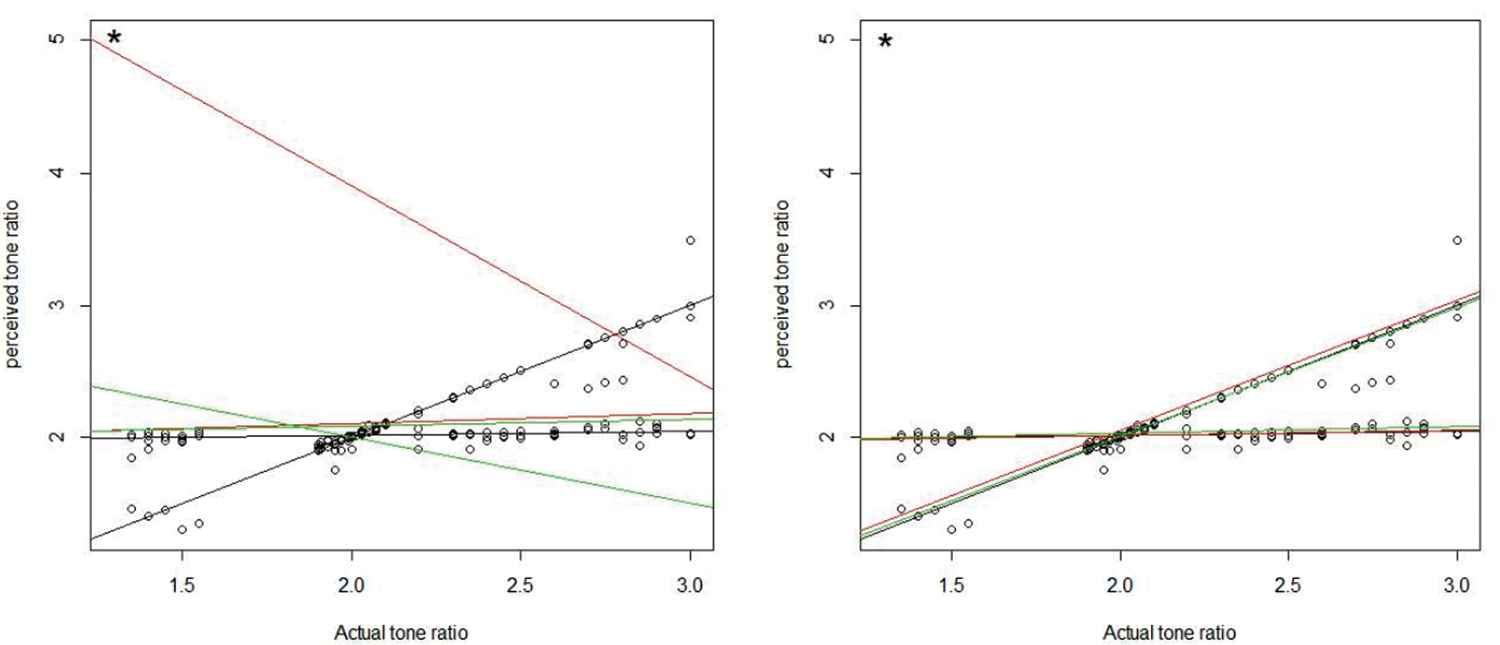
Mixture linear fitting with outlier (1.3,5). In left plot: black line-mixregs, green line-TLE, red line-MLE, in right plot: black line-mixregs, green line-bisquare, red line-mixregt.
From Table 6, we observe that the robust regression based on slash distribution is better than robust regression based normal and t distribution, according to the AIC [50] and BIC [51] criterion.
| Model | AIC | BIC | ||||||||||
|---|---|---|---|---|---|---|---|---|---|---|---|---|
| Normal | −0.039 | 1.008 | 1.892 | 0.056 | 0.084 | 0.084 | − | − | 0.325 | 107.257 | −200.513 | −179.439 |
| 0.006 | 0.998 | 1.978 | 0.017 | 0.011 | 0.011 | 1 | 1 | 0.485 | 202.804 | −387.608 | −360.513 | |
| Slash | 0.003 | 0.999 | 1.954 | 0.029 | 0.002 | 0.020 | 0.569 | 1.455 | 0.443 | 229.436 | −440.871 | −413.776 |
Fitted various models on the tone perception data set.
CONCLUSION
In this paper, we propose a robust MRM based on the slash distribution by extending the mixture of slash distributions to the regression setting. We suggest some guidelines to further improve the robustness of the proposed model against possible high leverage outliers by adaptively trimming high leverage points. The proposed method was compared to the traditional MLE and some other robust methods by using a simulation study and by using a real data set, it was shown that the results of the robust regression based on slash distribution is better than robust regression based normal and t distributions. Figure 2 also confirms this supremacy.
AUTHORS' CONTRIBUTIONS
The authors thank the Associate Editor and anonymous reviewers for their useful comments and suggestions on an earlier version of this manuscript which led to this improved one.
Funding Statement
This work has been conducted by University of Zabol.
APPENDIX A
APPENDIX B
APPENDIX C
REFERENCES
Cite this article
TY  - JOUR
AU  - Hadi Saboori
AU  - Ghobad Barmalzan
AU  - Mahdi Doostparast
PY  - 2020
DA  - 2020/04/09
TI  - Robust Mixture Regression Based on the Mixture of Slash Distributions
JO  - Journal of Statistical Theory and Applications
SP  - 118
EP  - 132
VL  - 19
IS  - 2
SN  - 2214-1766
UR  - https://doi.org/10.2991/jsta.d.200304.001
DO  - 10.2991/jsta.d.200304.001
ID  - Saboori2020
ER  -