
Modeling Vehicle Insurance Loss Data Using a New Member of T-X Family of Distributions
- DOI
- 10.2991/jsta.d.200421.001How to use a DOI?
- Keywords
- Heavy-tailed distributions; Weibull distribution; Insurance losses; Actuarial measures; Monte Carlo simulation; Estimation
- Abstract
In actuarial literature, we come across a diverse range of probability distributions for fitting insurance loss data. Popular distributions are lognormal, log-t, various versions of Pareto, log-logistic, Weibull, gamma and its variants and a generalized beta of the second kind, among others. In this paper, we try to supplement the distribution theory literature by incorporating the heavy tailed model, called weighted T-X Weibull distribution. The proposed distribution exhibits desirable properties relevant to the actuarial science and inference. Shapes of the density function and key distributional properties of the weighted T-X Weibull distribution are presented. Some actuarial measures such as value at risk, tail value at risk, tail variance and tail variance premium are calculated. A simulation study based on the actuarial measures is provided. Finally, the proposed method is illustrated via analyzing vehicle insurance loss data.
- Copyright
- © 2020 The Authors. Published by Atlantis Press SARL.
- Open Access
- This is an open access article distributed under the CC BY-NC 4.0 license (http://creativecommons.org/licenses/by-nc/4.0/).
1. INTRODUCTION
The usage of heavy tailed distributions for modeling insurance loss data is arguably an important subject matter for actuaries. Besides, one of the major goals of actuarial studies is to model the uncertainty pervading in the realm of insurance with respect to number of claims received in a particular period and the size of the claim severity. Generally speaking, insurance data sets are right-skewed [1], unimodal hump-shaped [2] and with heavy tails [3]. This type of heavy tailed distribution is apt for estimating insurance loss data and thereby helps in assessment of business risk level. Thus, due to its immense significance in actuarial sciences, this type of data has been studied extensively and several probability models have been proposed in actuarial literature. Among the variety of the models, the prominently used models related to insurance loss data, financial returns, file sizes on network servers, etc. are Pareto, lognormal, Weibull, gamma, log-logistic, Fréchet, Lomax, inverse Gaussian distributions; see Resnick [4], Hogg and Klugman [5], Qi [6], Hao and Tang [7], Gómez-Déniz and Calderín-Ojeda [8] and Calderín-Ojeda and Kwok [9] and Yang et al. [10], among others. For assessment of small size losses, distributions like log-normal, gamma, Weibull, Inverse Gaussian, etc. are used while for large insurance losses; commonly used distributions are Pareto, log-logistic, Fréchet, Lomax distributions, etc. Most of these aforementioned classical distributions are generalized for insurance loss data, financial returns etc. based on, but not limited to, the following five approaches: (i) transformation method, (ii) composition of two or more distributions, (iii) compounding of distributions, (iv) exponentiated distributions and (v) finite mixture of distributions, for further detail see, Miljkovic and Grün [11] and Bhati and Ravi [12].
In the recent past, Dutta and Perry [13] carried out an empirical study on loss distributions using Exploratory Data Analysis and empirical approaches to estimate the risk. However, due to lack of flexibility and poor results, they rejected the idea of using exponential, gamma and Weibull distributions and pointed out that “one would need to use a model that is flexible enough in its structure.”
Hence it is imperative to develop models either from the existing distributions or a new family of models to cater insurance loss data, financial returns, etc.
In the premises of the above, we are motivated to search for more flexible probability distributions which provide greater accuracy in data fitting. Hence, in this paper, we introduce a new member of the T-X family [14], called the weighted T-X(WT-X) family of distributions for modeling insurance losses. With this idea, we construct a new model named the weighted T-X Weibull (WT-XW) distribution which is more flexible than the Weibull distribution. We later prove empirically that the WT-XW model provides better fits than the well-known competitive distributions in terms of different measures of model validation by means of vehicle insurance loss data. Two of the competitive distributions have one extra model parameter, and the others have the same number of parameters.
We hope that the new distribution will attract wider applications in insurance loss data, financial returns, etc. Finally, estimation of the WT-XW model parameters using the method of maximum likelihood estimation have been carried out. Further, some actuarial measures such as value at risk (VaR), tail value at risk (TVaR), tail variance (TV) and tail variance premium (TVP) are also calculated.
The rest of the paper is organized as follows: In Section 2, we discuss the proposed approach based on the T-X family of distributions. In Section 3, the proposed approach is applied to the classical Weibull distribution to derive the WT-XW distribution. In Section 4, the maximum likelihood estimators (MLEs) of the parameters are derived and simulation study is carried out in the same section. Afterward, in Section 5, some of actuarial measures are obtained and numerical studies of the risk measures are provided. In Section 6, a numerical application is illustrated based upon the vehicle insurance loss data. Here, the weighted T-X Weibull distribution is compared with the Weibull and other (i) two-parameter distributions such as Pareto, Lomax, Burr X-II (BX-II), Log-normal and (ii) well-known three-parameter models such as Dagum and Marshall-Olkin Weibull (MOW) distributions under different discrimination and goodness of fit measures. Finally, some concluding remarks are given in the last section.
2. PROPOSED METHOD
Let
The cdf of the T-X family of distributions is defined by
Using the T-X family idea, several new classes of distributions have been introduced in the literature. Table 1 provides some
| Range of X | Members of T-X Family | |
|---|---|---|
| [0,1] | Beta-G [15] | |
| Gamma-G Type-2 [16] | ||
| Gamma-G Type-1 [17] | ||
| Gamma-G Type-3 [18] | ||
| Exponentiated T-X [19] | ||
| Logistic-G [20] | ||
| The Logistic-X Family [21] | ||
| New Weibull-X Family [22] | ||
| Weighted T-X Family(Proposed) |
Some members of the T-X family.
Now, we introduce the proposed family. Let
The density function corresponding to (2) is
If
The density function corresponding to (4) is
The key motivations for using the WT-XW distribution in practice are the following:
A very simple and convenient method to modify the existing distributions.
To improve the characteristics and flexibility of the existing distributions.
To introduce the extended version of the baseline distribution having closed form of distribution function.
To provide best fit to the heavy-tailed data in financial sciences and other related fields.
Another most important motivation of the proposed approach is to introduce new distributions without adding additional parameter results in avoiding re-scaling problems.
3. SUB-MODEL DESCRIPTION
In this section, we introduce a special sub-model of the proposed family, called the WT-XW distribution. Let
The pdf and hazard rate function (hrf) of the WT-XW model are given, respectively, by
For different values of the model parameters, plots of the density function of the WT-XW are sketched in Figure 1.
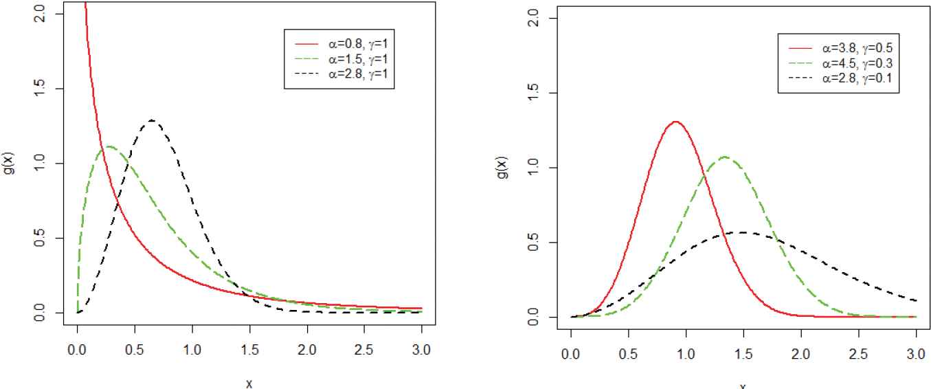
Different plots for the density function of the weighted T-X Weibull (WT-XW) distribution.
In Figure 1, we plotted different shapes for the density of WT-XW distribution for fixed values of
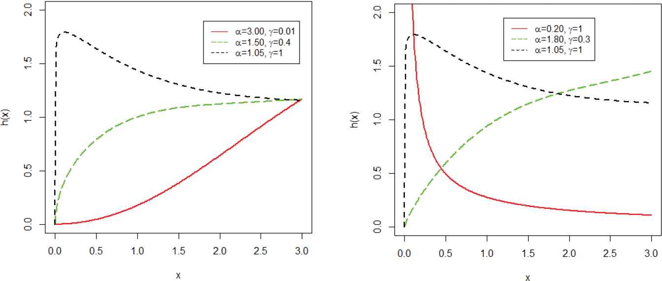
Different plots for the hrf of the weighted T-X Weibull (WT-XW) distribution.
4. ESTIMATION AND SIMULATION STUDY
Several methods for parameter estimation have been introduced in the literature. Among these approaches, the maximum likelihood method is the most commonly employed. The maximum likelihood estimations enjoy several desirable properties and can be used for constructing confidence intervals. In this section, the method of maximum likelihood estimation is used to estimate the model parameters
4.1. Maximum Likelihood Estimation
Here, we discuss the MLEs of the model parameters of the WT-XW distribution. Let
The log-likelihood function can be maximized either directly or by solving the nonlinear likelihood function obtained by differentiating (8). We used the goodness of fit function in R with “Nelder-Mead” algorithm to obtain the MLEs. The first order partial derivatives of (8) with respective to the parameters are given, respectively, by
Setting
4.2. Simulation Study
In order to assess the performances of the maximum likelihood estimates of the parameters of the proposed distribution, a comprehensive simulation study is carried out. The process is carried out as follows:
The number of Monte Carlo replications was made 500 times each with sample sizes
Initial values for the parameters are selected such as (i) for set 1,
Formulas used for calculating Bias and mean square error (MSE) are given by
Step (3) is also repeated for
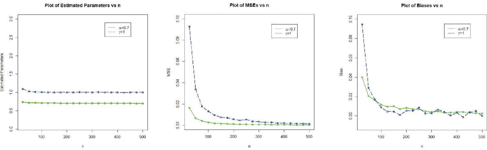
The simulation results are provided in Table 2 and displayed graphically in Figures 3–5.
| Set 1: α = 0.5, γ = 1 |
Set 2: α = 1.5, γ = 1 |
Set 3: α = 0.7, γ = 1 |
||||||||
|---|---|---|---|---|---|---|---|---|---|---|
| n | Par | MLE | Bais | MSE | MLE | Bais | MSE | MLE | Bais | MSE |
| 25 | 0.5387 | 0.03879 | 1.5829 | 0.0829 | 0.0771 | 0.7399 | 0.0399 | 0.0164 | ||
| 1.0674 | 1.0596 | 0.0596 | 0.0966 | 1.0943 | 0.0943 | 0.0926 | ||||
| 50 | 0.5197 | 0.01972 | 1.5534 | 0.0534 | 0.0350 | 0.7205 | 0.0205 | 0.0066 | ||
| 1.0166 | 1.0196 | 0.01961 | 0.0310 | 1.0288 | 0.0288 | 0.0337 | ||||
| 100 | 0.5104 | 0.01048 | 1.5264 | 0.0264 | 0.0163 | 0.7113 | 0.0113 | 0.0027 | ||
| 1.0032 | 1.0248 | 0.0248 | 0.0179 | 1.0087 | 0.0087 | 0.0132 | ||||
| 200 | 0.5031 | 0.00319 | 1.5111 | 0.0111 | 0.0067 | 0.7083 | 0.0083 | 0.0012 | ||
| 1.0028 | 1.0065 | 0.0065 | 0.0066 | 1.0052 | 0.0052 | 0.0057 | ||||
| 300 | 0.5012 | 0.00125 | 1.5025 | 0.0025 | 0.0041 | 0.7040 | 0.0040 | 0.0006 | ||
| 1.0001 | 1.0043 | 0.0043 | 0.0045 | 1.0027 | 0.0027 | 0.0033 | ||||
| 400 | 0.5004 | 0.00042 | 1.5030 | 0.0030 | 0.0031 | 0.7039 | 0.0039 | 0.0004 | ||
| 0.9998 | -1.0 |
0.9995 | −0.0004 | 0.0032 | 1.0031 | 0.0031 | 0.0019 | |||
| 500 | 0.5003 | 0.00036 | 1.5016 | 0.0016 | 0.0026 | 0.7024 | 0.0024 | 0.0002 | ||
| 1.0006 | 0.9995 | −0.0008 | 0.0030 | 0.9998 | −0.0001 | 0.0014 | ||||
WT-XW, weighted T-X Weibull; MLE, maximum likelihood estimator; MSE, mean square error.
The simulation results of the WT-XW distribution.
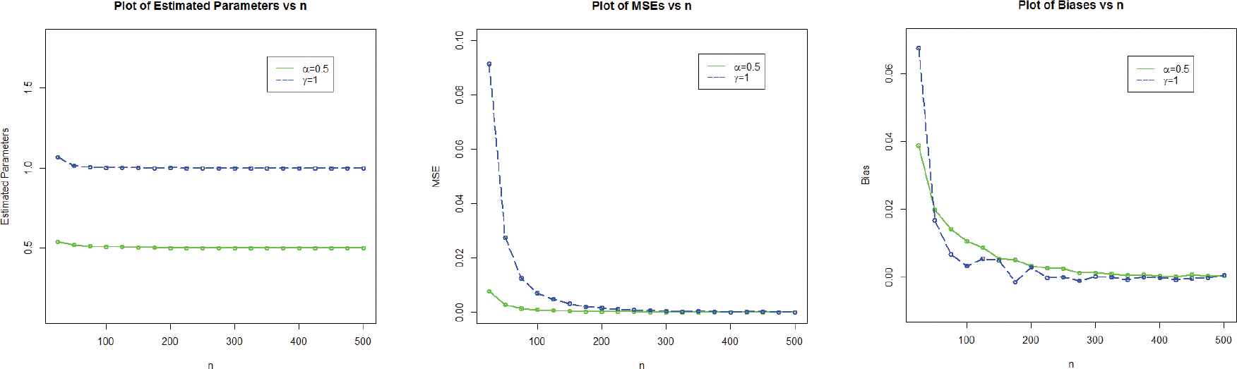
Graphical display of the simulation results of set 1.
Graphical display of the simulation results of set 3.
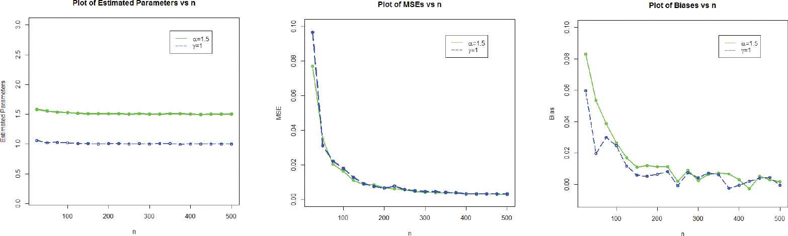
Graphical display of the simulation results of set 2.
5. ACTUARIAL MEASURES
One of the most important tasks of actuarial sciences institutions is to evaluate the exposure to market risk in a portfolio of instruments, which arise from changes in underlying variables such as prices of equity, interest rates or exchange rates. In this section, we calculate some important risk measures (VaR, TVaR, TV, TVP) for the proposed distribution, which play a crucial role in portfolio optimization under uncertainty.
5.1. Value at Risk
In the context of actuarial sciences, the measure VaR is widely used by practitioners as a standard financial market risk. It is also known as the quantile risk measure or quantile premium principle. The VaR is always specified with a given degree of confidence say
5.2. Tail Value at Risk
Another important measure is TVaR, also known as conditional tail expectation (CTE) or tail conditional expectation (TCE), used to quantifies the expected value of the loss given that an event outside a given probability level has occurred. Let X follows the proposed family, then TVaR of X is defined as
Recall, the definition of incomplete gamma function in the form
5.3. Tail Variance
The TV is one of the most important actuarial measures which pay attention to the TV beyond the VaR. The TV of the WT-XW distributed random variable is derived as
Consider
On solving, we get
Using (14) and (16) in (15), we get the expression for the TV of WT-XW distribution.
5.4. Tail Variance Premium
The TVP is another important measure play an essential role in insurance sciences. The TVP of WT-XW distributed random variable is derived as
5.5. Numerical Study of the Risk Measures
In this section, we simulate the risk measures described above to show the suitability of the proposed model. The simulation is performed for the Weibull and proposed model for the values of parameters. A model with higher values of the risk measures is said to have heavier tail. The simulated results provided in Tables 3 and 4 show that the proposed model has higher values of the risk measures than the traditional Weibull distribution. The simulation results are graphically displayed in Figures 6–9, which show that the proposed model has heavier tail than the Weibull distribution.
| Set 1: α = 0.7, γ = 0.5 |
|||||
|---|---|---|---|---|---|
| Dist | Level of Significance | VaR | TVaR | TV | TVP |
| 0.700 | 3.5226 | 8.8297 | 39.3627 | 18.6704 | |
| 0.750 | 4.3088 | 9.8157 | 41.3919 | 20.1637 | |
| 0.800 | 5.3327 | 11.070 | 43.8447 | 22.0318 | |
| Weibull | 0.850 | 6.7450 | 12.761 | 46.9629 | 24.5026 |
| 0.900 | 8.8951 | 15.276 | 51.2849 | 28.0976 | |
| 0.950 | 12.954 | 19.898 | 58.5092 | 34.5257 | |
| 0.975 | 17.440 | 24.889 | 65.5638 | 41.2805 | |
| 0.999 | 42.732 | 52.080 | 96.7712 | 76.2729 | |
| 0.700 | 1.7264 | 6.9464 | 65.3076 | 23.2733 | |
| 0.750 | 2.2581 | 7.9401 | 72.4397 | 26.0500 | |
| 0.800 | 3.0158 | 9.2719 | 81.6688 | 29.6892 | |
| WT-XW | 0.850 | 4.1748 | 11.179 | 94.3033 | 34.7551 |
| 0.900 | 6.1745 | 14.233 | 113.307 | 42.5602 | |
| 0.950 | 10.623 | 20.431 | 148.193 | 57.4798 | |
| 0.975 | 16.363 | 27.802 | 185.051 | 74.0656 | |
| 0.999 | 57.437 | 75.031 | 370.190 | 167.579 | |
WT-XW, weighted T-X Weibull; VaR, value at risk; TVaR, tail value at risk; TV, tail variance; TVP, tail variance premium.
Simulation results of VaR, TVaR, TV and TVP for
| Set 1: α = 1.3, γ = 1 |
|||||
|---|---|---|---|---|---|
| Dist | Level of Significance | VaR | TVaR | TV | TVP |
| 0.700 | 1.4266 | 5.7649 | 43.6476 | 16.6768 | |
| 0.750 | 1.8914 | 6.5885 | 48.3030 | 18.6643 | |
| 0.800 | 2.5493 | 7.6857 | 54.3512 | 21.2735 | |
| Weibull | 0.850 | 3.5421 | 9.2447 | 62.7181 | 24.9243 |
| 0.900 | 5.2180 | 11.718 | 75.5996 | 30.6186 | |
| 0.950 | 8.8325 | 16.697 | 100.570 | 41.8403 | |
| 0.975 | 13.392 | 22.622 | 129.265 | 54.9384 | |
| 0.999 | 46.962 | 62.527 | 311.306 | 140.354 | |
| 0.700 | 0.4150 | 4.6755 | 119.152 | 34.4637 | |
| 0.750 | 0.6220 | 5.5085 | 138.819 | 40.2133 | |
| 0.800 | 0.9619 | 6.6914 | 166.526 | 48.3229 | |
| WT-XW | 0.850 | 1.5702 | 8.5105 | 208.787 | 60.7074 |
| 0.900 | 2.8319 | 11.708 | 282.440 | 82.3183 | |
| 0.950 | 6.4148 | 19.165 | 452.656 | 132.329 | |
| 0.975 | 12.300 | 29.521 | 688.040 | 201.531 | |
| 0.999 | 81.598 | 124.89 | 2925.11 | 856.172 | |
WT-XW, weighted T-X Weibull; VaR, value at risk; TVaR, tail value at risk; TV, tail variance; TVP, tail variance premium.
Simulation results of VaR, TVaR, TV and TVP for
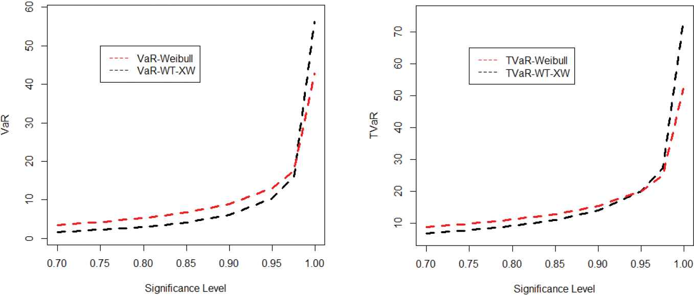
Plots for the value at risk (VaR) and tail value at risk (TVaR) of the Weibull and weighted T-X Weibull (WT-XW) distributions.
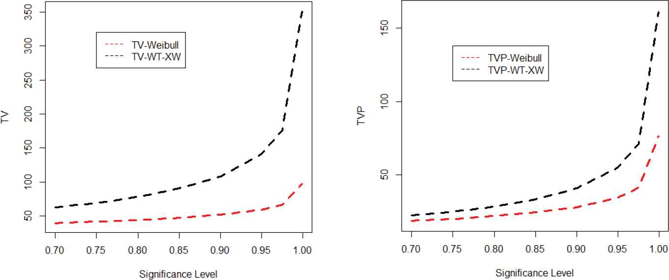
Plots for the tail variance (TV) and tail variance premium (TVP) of the Weibull and weighted T-X Weibull (WT-XW) distributions.
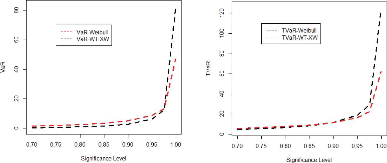
Plots for the value at risk (VaR) and tail value at risk (TVaR) of the Weibull and weighted T-X Weibull (WT-XW) distributions.
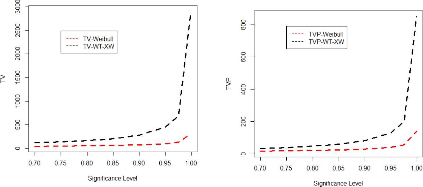
Plots for the tail variance (TV) and tail variance premium (TVP) of the Weibull and weighted T-X Weibull (WT-XW) distributions.
The simulation process is described below:
Random samples of sizes
1000 repetitions are made to calculate the VaR, TVaR, TV and TVP for these distributions.
6. A REAL-LIFE APPLICATION
The main applications of the heavy tail models are the so-called extreme value theory or insurance loss phenomena. We consider a data set from insurance sciences. In this section, we illustrate the WT-XW model by analyzing vehicle insurance loss data to show how the proposed method works in practice. Furthermore, we calculate the actual measures of the Weibull and WT-XW distributions using the real data set.
6.1. Application to the Vehicle Insurance Loss Data
In this sub-section, we illustrate the proposed method using a real data set representing the vehicle insurance losses available at http://www.businessandeconomics.mq.edu.au/our_departments/Applied_Finance_and_Actuarial_Studies/research/books/GLMsforInsuranceData. First, we check whether the considered data set actually comes from the WT-XW or not by goodness of fit test and compare the fits with the other heavy tailed distributions including the two and three parameters distributions. This procedure is based on the Anderson Darling (AD) test statistic, Cramer–von-Mises (CM) test statistic and Kolmogorov–Smirnov (KS) statistic with the corresponding p-values. Note that, the AD, CM and KS statistic to be used only to verify the goodness-of-fit and not as a discrimination criteria. Therefore, we consider four discrimination criteria based on the log-likelihood function evaluated at the maximum likelihood estimates. The criteria are Akaike information criterion (AIC), Bayesian information criterion (BIC), Hannan-Quinn information criterion (HQIC), Corrected Akaike information criterion (CAIC). A model with lowest values for these statistics could be chosen as the best model to fit the data. The analytical measures are calculated are calculated as follows:
The AD test statistic is given by
The CM test statistic is given by
The KS test statistic is given by
The AIC is given by
The BIC is given by
The HQIC is given by
The CAIC is given by
Weibull
Pareto
Lomax
B-XII
Log-normal
Dagum
MOW
The values of MLEs of the parameters along with the corresponding standard errors (in parenthesis) are provided in Table 5. The discrimination criteria are presented in Table 6. Whereas, the goodness of fit measures are reported in Table 7. A model with lowest values for these statistics is considered as a best candidate model. As we see, the results (Tables 6 and 7) show that the WT-XW distribution provides better fit than the other considered competitors. Hence, the proposed model can be used as a best candidate model for modeling insurance losses. Furthermore, in support of Tables 6 and 7, the estimated cdf and pdf of the proposed model are plotted in Figure 10. The Kaplan–Meier survival plot and PP plot are provided in Figure 11. These plots also reveal that the WT-XW distribution provides the best fit to data compared to the other models.
| Dist. | |||||||
|---|---|---|---|---|---|---|---|
| WT-XW | 0.868 (0.038) | 0.006 (0.001) | – | – | – | – | – |
| Weibull | 0.759 (0.041) | 0.019 (0.005) | |||||
| Pareto | 0.959 (0.291) | 1.385 (0.491) | – | – | – | – | – |
| Lomax | 1.689 (0.357) | 1.256 (0.648) | – | – | – | – | – |
| B-XII | – | – | – | 6.672 (11.259) | 0.032 (0.055) | – | – |
| Log-normal | – | – | 0.965 (0.325) | – | – | – | 0.765 (0.101) |
| Dagum | 0.968 (0.040) | 0.903 (0.103) | – | – | – | 0.698 (0.795) | – |
| MOW | 0.594 (0.098) | 0.072 (0.289) | 2.515 (0.904) | – | – | – | – |
WT-XW, weighted T-X Weibull; MOW, Marshall-Olkin Weibull.
The estimated values of the parameters with standard errors in parenthesis) of the fitted distributions.
| Dist. | AIC | BIC | CAIC | HQIC |
|---|---|---|---|---|
| WT-XW | 2234.262 | 2240.603 | 2234.331 | 2236.833 |
| Weibull | 2243.208 | 2249.549 | 2243.277 | 2245.780 |
| Pareto | 2260.071 | 2276.518 | 2266.090 | 2264.057 |
| Lomax | 2272.037 | 2279.289 | 2274.980 | 2273.885 |
| B-XII | 2499.052 | 2505.393 | 2499.121 | 2501.624 |
| Lognormal | 2236.643 | 2243.980 | 2237.873 | 2239.098 |
| Dagum | 2238.876 | 2245.084 | 2239.764 | 2240.709 |
| MOW | 2256.673 | 2266.184 | 2256.812 | 2260.530 |
WT-XW, weighted T-X Weibull; MOW, Marshall-Olkin Weibull; AIC, Akaike information criterion; BIC, Bayesian information criterion; HQIC, Hannan-Quinn information criterion; CAIC, Corrected Akaike information criterion.
Analytical measures of the proposed and other competitive models.
| Dist. | CM | AD | KS | p-value |
|---|---|---|---|---|
| WT-XW | 0.595 | 3.659 | 0.090 | 0.152 |
| Weibull | 0.724 | 4.399 | 0.103 | 0.123 |
| Pareto | 1.103 | 5.709 | 0.478 | 0.101 |
| Lomax | 1.290 | 5.774 | 0.573 | 0.098 |
| B-XII | 0.809 | 5.107 | 0.408 | 0.118 |
| Log-normal | 0.635 | 3.971 | 0.094 | 0.139 |
| Dagum | 0.6409 | 4.094 | 0.095 | 0.134 |
| MOW | 0.903 | 5.431 | 0.421 | 0.109 |
WT-XW, weighted T-X Weibull; MOW, Marshall-Olkin Weibull; Anderson Darling (AD) test statistic, CM, Cramer von-Mises; KS, Kolmogorov-Smirnov.
Analytical measures of the proposed and other competitive models.
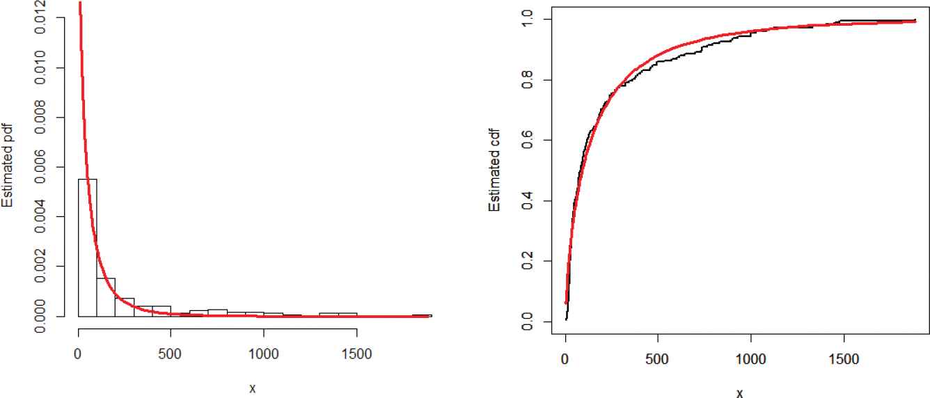
Estimated probability density function (pdf) and cumulative distribution function (cdf) of the weighted T-X Weibull (WT-XW) distribution.
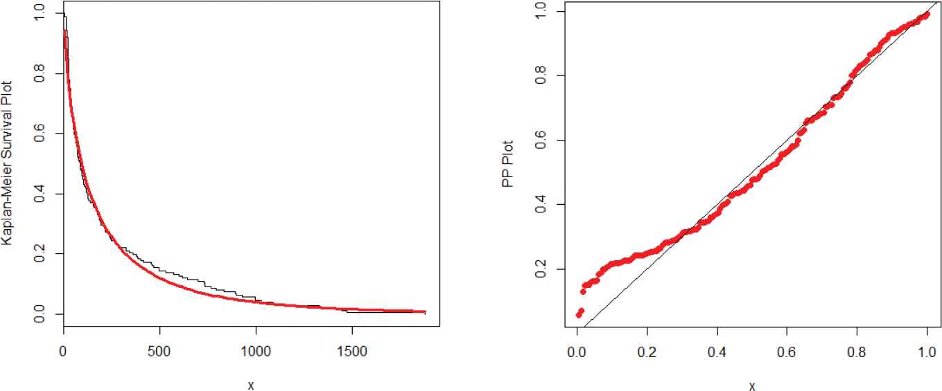
Kaplan–Meier survival and PP-plots of the weighted T-X Weibull (WT-XW) distribution.
6.2. Calculation of the Actuarial Measures Using the Vehicle Insurance Loss Data
In this sub-section, we calculate the actuarial measures of the Weibull and the WT-XW distribution using the estimated values of the parameters for the insurance loss data set. The numerical results are reported in Table 8.
| Dist | Parameters | Level of Significance | VaR | TVaR | TV | TVP |
|---|---|---|---|---|---|---|
| 0.700 | 255.920 | 590.031 | 142719.084 | 36269.802 | ||
| 0.750 | 308.244 | 651.818 | 148310.999 | 37729.568 | ||
| 0.800 | 375.326 | 729.705 | 154963.790 | 39470.652 | ||
| Weibull | 0.850 | 466.263 | 833.533 | 163268.542 | 41650.669 | |
| 0.900 | 602.016 | 985.866 | 174526.532 | 44617.499 | ||
| 0.950 | 851.889 | 1260.832 | 192776.813 | 49455.035 | ||
| 0.975 | 1121.071 | 1552.087 | 210014.124 | 54055.618 | ||
| 0.999 | 2564.815 | 3075.459 | 281148.054 | 73362.473 | ||
| 0.700 | 258.291 | 639.741 | 210718.724 | 53319.422 | ||
| 0.750 | 312.536 | 710.832 | 222490.325 | 56333.413 | ||
| 0.800 | 383.825 | 801.937 | 236506.473 | 59928.555 | ||
| WT-XW | 0.850 | 483.543 | 925.725 | 253773.605 | 64369.126 | |
| 0.900 | 638.454 | 1111.378 | 276269.591 | 70178.776 | ||
| 0.950 | 938.583 | 1454.882 | 309257.870 | 78769.349 | ||
| 0.975 | 1275.602 | 1824.653 | 335843.672 | 85785.571 | ||
| 0.999 | 3111.461 | 3740.299 | 413793.771 | 107188.742 |
WT-XW, weighted T-X Weibull; VaR, value at risk; TVaR, tail value at risk; TV, tail variance; TVP, tail variance premium.
Simulation results of VaR, TVaR, TV and TVP for
As we have mentioned earlier that a model with higher values of the risk measures is said to posses the heavier tails. From the numerical results for the actuarial measures of the proposed and Weibull distributions provided in Table 6, it is clear that the proposed distribution has heavier tail than the Weibull distribution and can be used as good candidate model for modeling heavy tailed insurance data sets.
7. CONCLUDING REMARKS
In the present work, we have proposed a versatile two parameter heavy tailed weighted T-X family of the Weibull distribution. The distribution has closed-form expressions for some insurance measures such as VaR, TVaR, TV and TVP. We have also studied some of its basic properties. Although the method has only been applied to the classical Weibull distribution, yet, this procedure can be extended by using other probabilistic families as parent distribution. The motivation for conducting this study is to find out whether the model can be applied in respect of vehicle insurance loss data. Numerical results show that the WT-XW distribution outperforms other existing long-tail distributions under the different measures of model assessment considered in respect of vehicle insurance loss data. This new method, which has a promising approach for data modeling in the actuarial field, may be very useful for practitioners who handle large claims and thereby it can be deemed as an alternative to the Weibull distribution.
AUTHORS' CONTRIBUTIONS
(i) Zubair Ahmad wrote the initial draft of the paper and did the simulation study and analysis, (ii) Eisa Mahmoudi helped in the simulation study and superivised overall work, and (iii) Sanku Dey and Saima K. Khosa helped in writing and improving the Introduction Section.
FUNDING STATEMENT
The work is sponsored by the Department of Statistics, Yazd University, Iran.
DATA AVAILABILITY STATEMENT
This work is mainly a methodological development and has been applied on secondary data related to the Vehicle Insurance Loss Data, but if required, data will be provided.
ACKNOWLEDGMENT
The authors are grateful to the Editor and referees for many of their valuable comments and suggestions which lead to this improved version of the manuscript. The first two authors also acknowledge the support of the Yazd University, Iran.
DEDICATION
This article is drafted from the Ph.D work of the first Author. The author would like to dedicate this article to the memory of his late parents.
APPENDIX
R Code for calculating the analysis measures in this manuscript.
############################################################
Important Note:
The data is saved in the csv file in our PC, so we used the commond
“read.csv” to load the data in to R. The data is saved in column 11,
that's why we have used the commond “data=data[,11]” to call the
data from the 11th column of the csv file. In the propogram, pm is
used for the proposed model.
############################################################
data<-read.csv(file.choose(), header=TRUE)
data=data[,11]
data=data[!is.na(data)]
data=data/5
data
############################################################
##### The density of the proposed distribution
############################################################
pdf_pm <- function(par,x)
{
alpha=par[1]
gamma=par[2]
alpha*gamma*(x^(alpha-1))*exp(-gamma*x^alpha)*(1+exp (-gamma*x^alpha))
*(1/(exp(1-exp(-gamma*x^alpha))))
}
############################################################
##### The distribution function of the proposed distribution
############################################################
cdf_pm <- function(par,x)
{
alpha= par[1]
gamma= par[2]
1-(exp(-gamma*x^alpha)/(exp(1-exp(-gamma*x^alpha))))
}
set.seed(0)
goodness.fit(pdf=pdf_pm, cdf=cdf_pm,
starts = c(0.5,0.5), data = data,
method=“Nelder-Mead”, domain=c(0,Inf),mle=NULL)
REFERENCES
Cite this article
TY  - JOUR
AU  - Zubair Ahmad
AU  - Eisa Mahmoudi
AU  - Sanku Dey
AU  - Saima K. Khosa
PY  - 2020
DA  - 2020/05/28
TI  - Modeling Vehicle Insurance Loss Data Using a New Member of T-X Family of Distributions
JO  - Journal of Statistical Theory and Applications
SP  - 133
EP  - 147
VL  - 19
IS  - 2
SN  - 2214-1766
UR  - https://doi.org/10.2991/jsta.d.200421.001
DO  - 10.2991/jsta.d.200421.001
ID  - Ahmad2020
ER  -