
Empirical Estimation for Sparse Double-Heteroscedastic Hierarchical Normal Models
- DOI
- 10.2991/jsta.d.200422.001How to use a DOI?
- Keywords
- Asymptotic optimality; Heteroscedasticity; Empirical estimators; Sparsity; Stein's unbiased risk estimate (SURE)
- Abstract
The available heteroscedastic hierarchical models perform well for a wide range of real-world data, but for the data sets which exhibit heteroscedasticity mainly due to the lack of constant means rather than unequal variances, the existing models tend to overestimate the variance of the second level model which in turn will cause substantial bias in the parameter estimates. Therefore, in this study, we develop heteroscedastic hierarchical models, called double-heteroscedastic hierarchical models, that take into account the heterogeneity in the means for the second level of the models, in addition to considering the heterogeneity of variance for the first level of the models. In these models, we assume that the vector of means in the second level is sparse. We derive Stein's unbiased risk estimators (SURE) for the parameters in the model based on data decomposition and study their risk properties both in theory and in numerical experiments under the squared loss. The comparison between our SURE estimator and the classical estimators such as empirical Bayes maximum likelihood estimator (EBMLE) and empirical Bayes moment estimator (EBMOM) is illustrated through a simulation study. Finally, we apply our model to a Baseball data set.
- Copyright
- © 2020 The Authors. Published by Atlantis Press SARL.
- Open Access
- This is an open access article distributed under the CC BY-NC 4.0 license (http://creativecommons.org/licenses/by-nc/4.0/).
1. INTRODUCTION
Hierarchical models have been extensively studied and widely used in many disciplines such as biology, climatology, ecology, medicine and engineering. A hierarchical model is a multi-level model which integrates information from different sources to achieve coherent inferences of unknowns (e.g., [1–3]). Among the many statisticians who have made significant contribution to theories and applications of hierarchical models, James and Stein [4] and Stein [5] were pioneers by studying simultaneous statistical inferences for the mean of several normal populations. The joint work of James and Stein has fundamentally increased the use of hierarchical models in recent decades. Stein's shrinkage estimators that had an interesting empirical Bayes interpretation were the basis for developing shrinkage estimation in multilevel normal models. Later, Efron and Morris [6] showed further implications of Stein's shrinkage estimator and proposed several competing parametric empirical Bayes estimators.
To date, both parametric and nonparametric empirical Bayes properties of shrinkage estimators have been extensively studied under either a homoscedastic (equal subpopulation variances) or heteroscedastic (unequal subpopulation variances) assumption. For more details, see Berger and Strawderman [7] and Brown and Greenshtein [8]. The majority of these investigations have focused on the risk properties of estimators with various loss functions. For example, the admissible minimax estimators for homoscedastic hierarchical normal models with usual quadratic loss functions were considered by Baranchik [9], a class of proper Bayes minimax estimators was studied by Strawderman [10], and a sufficient condition for admissibility of generalized Bayes estimators was investigated by Brown [11]. Comparisons between those estimators under different loss functions are discussed in Brown [12], Berger [13] and Berger and Strawderman [7].
Recently, heteroscedastic hierarchical normal models have received more attention due to the demand for real applications. Xie et al. [14] proposed a class of shrinkage estimators based on Stein's unbiased risk estimate (SURE) and studied the asymptotic properties of various common estimators as the number of means to be estimated increases. In particular, they established the asymptotic optimality property for the SURE estimators. They further extended their estimators to a class of semi-parametric shrinkage estimators and established corresponding asymptotic optimality results. Ghoreishi and Meshkani [15] considered the estimation of a set of normal population means by assuming heteroscedasticity in both levels of a two-level hierarchical model. They developed weighted shrinkage estimators of population means based on weighted SURE. This is achieved by first estimating the nuisance parameters of variances and then using them in the derivation of the shrinkage estimators of means. Still in the context of heteroscedastic models, Xie et al. [16] discussed the simultaneous inference of mean parameters in a family of distributions with quadratic variance function. They studied the asymptotic optimality properties of their semi-parametric/parametric shrinkage estimators that were defined for the location-scale family and the natural exponential family. Ghoreishi [17] studied the Bayesian analysis of a fully heteroscedastic hierarchical model. He used a class of local-global shrinkage priors, Dirichlet–Laplace priors and evaluated the optimal posterior concentration of their corresponding Bayes estimators.
Compared to nonparametric Bayes estimators, parametric empirical Bayes estimators are more commonly used in real data analysis [18]. The application of parametric empirical Bayes usually involves unknown hyper-parameters that need to be estimated. The empirical Bayes maximum likelihood estimator (EBMLE), empirical Bayes moment estimator (EBMOM) and SURE are the common approaches for the hyper-parameter estimation, see Brown [19] and references therein.
Although in general the available heteroscedastic hierarchical models perform well for a wide range of real-world data, they may fit poorly for the data sets which exhibit heteroscedasticity mainly due to the lack of constant means rather than unequal variances. For such data, implementation of the existing heteroscedastic hierarchical models tends to overestimate the variance of the second-level model which will cause substantial bias in the parameter estimates. According to the above description, the present study is an attempt to consider the following points
We develop heteroscedastic hierarchical models that take into account the heterogeneity in the means for the second-level of the model, in addition to considering the heterogeneity of variance for the first level of the models. We call these extended models as “double-heteroscedastic hierarchical models.”
Throughout the paper, we assume that the vector of the second level means is a sparse vector. So, we derive SURE for the parameters in the model based on data decomposition and study their risk properties both in theory and in numerical experiments under the squared loss. The comparison between our SURE estimator and the classical estimators such as EBMLE and EBMOM is illustrated through a simulation study.
Practically, our sparse double-heteroscedastic hierarchical models can be widely used in signal detection and gene effect studies. For example, when many gene families (a group of homologous genes which they share similar sequences and they may have identical functions) are compared for the healthy and treated groups, only a few of these sequences are detected, which are known to cause the disease. Here, the sparse double-heteroscedastic hierarchical models perform well for this comparison.
In the application section, we apply our model to the baseball data analyzed by Brown [19] and compare the batting average of two halves for each player and, finally, detect the players who have had different performances in two halves of the baseball season.
The paper is structured as follows: In section 2, we first give preliminaries including notations and definitions, then introduce a two-level sparse heteroscedastic hierarchical model. Section 3 derives estimators for all parameters in the hierarchical model, and Section 4 studies their risk properties. Extensive stimulation studies for evaluation of our parameter estimates are given in Section 5 and a data example of applying our model is presented in Section 6, followed by a brief discussion in Section 7. Technical proofs are given in the Appendix.
2. PRELIMINARIES
2.1. Notations and Definitions
Given a vector
2.2. Two-Level Sparse Heteroscedastic Hierarchical Normal Model
Let
We further assume that the vector
From model (2.1) and using Bayes' theorem, we have the posterior distribution of
We opt for the posterior mode to be a class of shrinkage estimators for
Since the usual heteroscedastic hierarchical models are derived based on model (2.1) but with conditions
3. EMPIRICAL PARAMETER ESTIMATORS OF HYPER-PARAMETERS
We introduce empirical methods for estimating the hyper-parameters in model (2.1). We will start with the empirical methods for estimating the hyper-parameter
3.1. Empirical Estimators of λ
Although empirical approaches such as EBMLE and EBMOM have been frequently used to estimate the model hyper-parameters, we aim to use SURE to estimate the hyper-parameter
From (2.1), the marginal distribution of
Let
It is easy to verify that
By Lemma 1 in Carpentier and Verzelen [20], it is straightforward to see that for some constant
For more details on the proof and the
Consequently, a range of the empirical estimate for
If we are interested in estimating
Or, if we are interested in an EBMLE estimator of
We however focus on estimating
Under this loss function and using (2.2), the shrinkage estimator
If we define
For more details see Xie et al. [14] and Ghoreishi and Meshkani [15].
3.2. Empirical Sparsity Estimation
The estimation of sparsity
We then employ the above approximation to estimate
To derive the estimator, we first consider the empirical characteristic function of
Then we define a statistic
It is straightforward to see that
In addition, we may be interested in constructing an
It is easy to verify that for a given
Note that since
Given
We propose the following iterative procedure for practical purpose:
Randomly choose half of the sample as our initial estimate of
Randomly choose 5% of the observations in
Repeat Step 1 until
The justification of the proposed iterative estimation procedure is stated in the following proposition:
3.3. Empirical Estimation of α i
To estimate the hyper-parameters
An unbiased estimator for the risk
Given empirical estimates
4. RISK PROPERTIES OF SURE ESTIMATOR
We establish properties of the SURE estimator in (3.16) under the following squared-loss function that is applied to the entire data:
For ease of notation, in the following we assume
This decomposition allows us to evaluate the performance of the SURE estimators using estimators derived based on partial data, that is,
The following theorem shows how well
Theorem 4.1.
Under Conditions C1 and C2 in the Appendix, we have
The proof of this theorem is deferred to the Appendix.
5. NUMERICAL STUDIES
We carry out simulation studies to evaluate the performance of the SURE estimators for sparse heteroscedastic hierarchical normal models. To measure the performance of the estimators, we compute the risk
Scenario I: Baseline model
Scenario II: Assume a two-component mixture model for
Scenario II introduces a more complex mean structure than Scenario I.
Scenario III: Assume a three-component mixture model for
Scenario IV: Assume three-component mixture models for both
Scenario IV has a more complex variance structure than Scenarios I-III.
For each simulated data, we estimate the hyper-parameters
Using this criterion, we find
To evaluate the performance of our estimators, we consider the oracle estimator of
In addition to the oracle estimator, we also compute the EBMOM and EBML estimates and their MCR, ECP and risk. The summary of simulation results over 200 runs is reported in Table 1. In particular, we show the variability of
| Scenarios | Method | MCR | ECP | |||
|---|---|---|---|---|---|---|
| Oracle | 0.401 (0.023) | 9.421 (3.09) | 0.137 (0.083) | 0.70 (0.173) | 0.217 | |
| Scenario I | SURE | 0.404 (0.043) | 9.381 (3.24) | 0.191 (0.092) | 0.63 (0.173) | 0.249 |
| EBMOM | 0.513 (0.058) | 3.299 (3.41) | 0.671 (0.173) | 0.21 (0.121) | 0.734 | |
| EBMLE | 0.627 (0.067) | 0.632 (4.33) | 0.819 (0.192) | 0.08 (0.114) | 1.117 | |
| Oracle | 0.401 (0.022) | 7.948 (3.19) | 0.212 (0.108) | 0.66 (0.165) | 0.422 | |
| Scenario II | SURE | 0.401 (0.023) | 7.700 (3.32) | 0.241 (0.123) | 0.61 (0.154) | 0.437 |
| EBMOM | 0.592 (0.051) | 1.890 (3.89) | 0.757 (0.208) | 0.14 (0.102) | 0.801 | |
| EBMLE | 0.693 (0.055) | 0.860 (3.61) | 0.901 (0.203) | 0.02 (0.093) | 1.115 | |
| Oracle | 0.402 (0.027) | 9.808 (3.27) | 0.163 (0.099) | 0.66 (0.163) | 0.267 | |
| Scenario III | SURE | 0.403 (0.027) | 9.592 (3.35) | 0.182 (0.104) | 0.64 (0.160) | 0.298 |
| EBMOM | 0.601 (0.057) | 3.978 (3.48) | 0.610 (0.123) | 0.22 (0.123) | 0.721 | |
| EBMLE | 0.617 (0.056) | 1.154 (3.62) | 0.857 (0.173) | 0.07 (0.099) | 1.112 | |
| Oracle | 0.401 (0.023) | 8.883 (3.11) | 0.220(0.008) | 0.65(0.176) | 0.333 | |
| Scenario IV | SURE | 0.403 (0.026) | 8.576 (3.23) | 0.236(0.008) | 0.61(0.142) | 0.421 |
| EBMOM | 0.577 (0.054) | 5.396 (3.88) | 0.498(0.049) | 0.42(0.133) | 0.877 | |
| EBMLE | 0.611 (0.051) | 3.479 (4.64) | 0.619(0.058) | 0.24(0.114) | 1.234 |
EBMLE, empirical Bayes maximum likelihood estimator; EBMOM, empirical Bayes maximum likelihood estimator; SURE, Stein's unbiased risk estimate; MCR, misclassification rate; ECP, empirical coverage probability.
Simulation results under various scenarios. The columns of
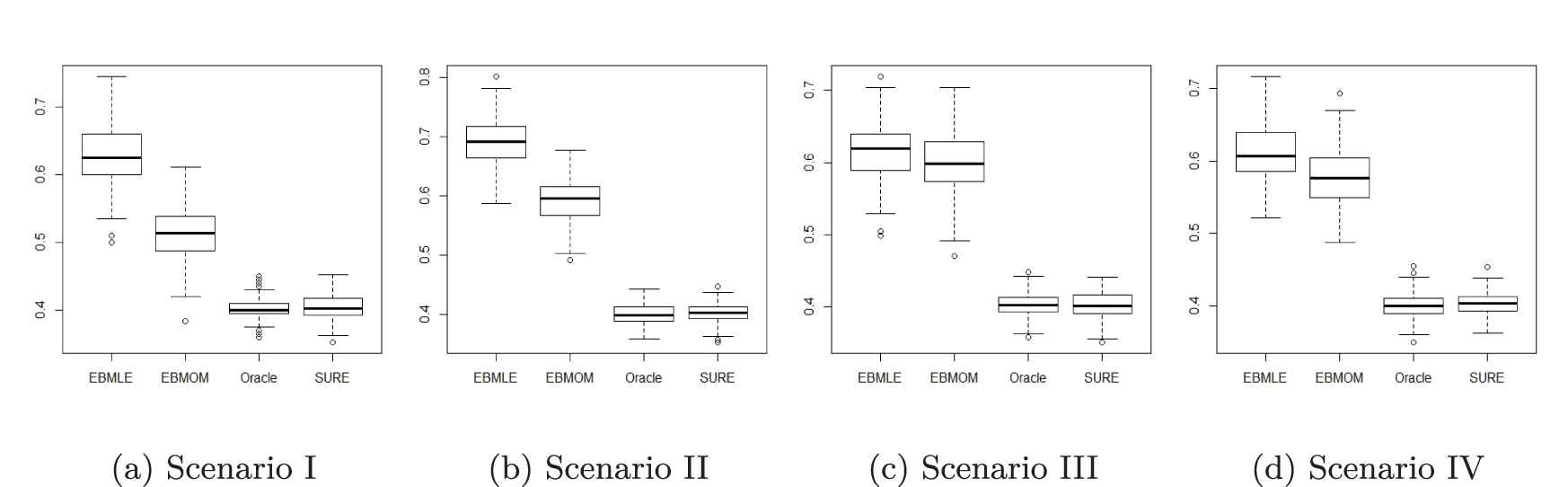
Boxplots for
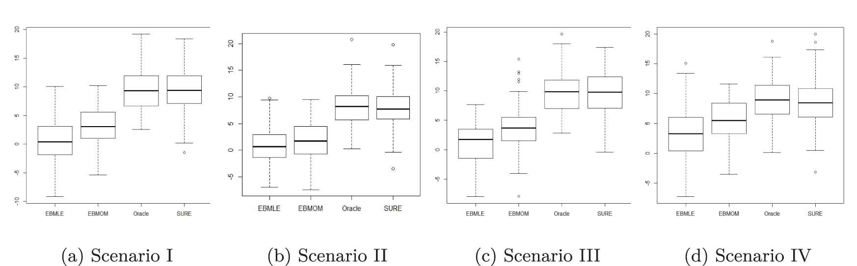
Boxplots for
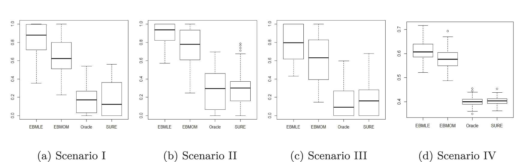
Boxplots for MCR with EBMLE, EBMOM, Oracle and SURE methods for four scenarios.
To examine whether the true sparsity of the data affects the sparsity parameter estimation, we rerun the simulation by setting
| 10 | 15 | 20 | 30 | 50 | ||
|---|---|---|---|---|---|---|
| 9.381 | 13.612 | 18.704 | 28.375 | 46.441 | ||
| Scenario-I | ECP | 0.63 | 0.60 | 0.71 | 0.68 | 0.44 |
| MCR | 0.187 | 0.146 | 0.104 | 0.077 | 0.078 | |
| 7.700 | 11.890 | 15.658 | 24.276 | 40.442 | ||
| Scenario-II | ECP | 0.61 | 0.50 | 0.44 | 0.31 | 0.19 |
| MCR | 0.282 | 0.243 | 0.228 | 0.194 | 0.191 | |
| 9.592 | 14.705 | 18.892 | 19.284 | 19.709 | ||
| Scenario-III | ECP | 0.64 | 0.62 | 0.69 | 0.14 | 0.11 |
| MCR | 0.177 | 0.113 | 0.357 | 0.676 | 0.605 | |
| 8.576 | 13.632 | 17.482 | 17.574 | 17.681 | ||
| Scenario-IV | ECP | 0.61 | 0.67 | 0.56 | 0.09 | 0.05 |
| MCR | 0.238 | 0.142 | 0.159 | 0.414 | 0.646 | |
SURE, Stein's unbiased risk estimate; MCR, misclassification rate; ECP, empirical coverage probability.
Estimation of
6. APPLICATION TO REAL DATA
We analyze the baseball data that was first introduced by Brown [19] and then later analyzed by Xie et al. [14]. This dataset contains batting records for all Major League Baseball players in the season of 2005. We first divide the dataset into two half seasons, then our goal is to compare the batting average of two halves for each player and detect the players who have had different performance in two halves of the baseball season. Following Brown [19] and Xie et al. [14], we removed the players whose number of at-bats is less than 10 to improve the accuracy of estimation. After this screening procedure, only 503 players out of 929 were selected.
Following the notations in Brown [19] and Xie et al. [14], we use
Our analysis assumes independency between the performance of each player in two half seasons. This assumption may seem unreasonable at first glance. However, if we look at the performance of each player in two half-seasons, the Yule association measure, defined as
The cross-validation yields
| Full Name | Pitchers (1)/Nonpitchers (0) | ||||||
|---|---|---|---|---|---|---|---|
| Magglio Ordonez | 0 | 10 | 208 | 0 | 92 | 2.716 | 0.4379 |
| Brandon Webb | 1 | 27 | 35 | 0 | 6 | 2.622 | 0.3375 |
| Victor Martinez | 0 | 252 | 442 | 61 | 106 | 2.864 | 0.1281 |
| Todd Helton | 0 | 269 | 414 | 71 | 92 | 2.769 | 0.1278 |
| Rafael Furcal | 0 | 304 | 507 | 71 | 104 | 2.625 | 0.1109 |
| Aaron Hill | 0 | 131 | 273 | 47 | 52 | 2.609 | 0.0258 |
| Moises Alou | 0 | 225 | 341 | 73 | 37 | −3.257 | −0.1632 |
| Desi Relaford | 0 | 175 | 210 | 45 | 2 | −2.976 | −0.2781 |
| Tony Blanco | 0 | 44 | 56 | 11 | 0 | −2.921 | −0.4202 |
Information of the 10 players and their
7. DISCUSSION
We develop heteroscedastic hierarchical normal models with sparse and unequal mean as well as derive SURE for such models at demand of the data sets which exhibit heteroscedasticity mainly due to the lack of constant means rather than unequal variances. Our model fills in the gap that no existing literatures are devoted to the heteroscedastic hierarchical normal models with sparse and unequal mean structure. Both theory and simulation study show that our SURE holds nice properties and outperforms the classic EBML and EBMOM estimator for our proposed model. However, we also notice that the SURE estimates are sensitive to the mean and variance structures as the sparsity decreases. We leave the investigation on improving parameter estimates for future research.
ACKNOWLEDGMENTS
We wish to thank the editor and two anonymous referees whose comments greatly improved the article.
APPENDIX
To establish the asymptotic results, we assume two mild conditions following Ghoreishi and Meshkani [15] and Xie et al. [14],
- C1)
- C2)
Moreover, without loss of generality, we assume that the sub-populations were re-indexed such that we have
Proof of Proposition 3.1
Define
That is,
Proof of Theorem 4.1
Consider the squared-loss function
It is easy to see that the corresponding risk function of this loss function is given by
The SURE unbiased estimator of
For a given
Hence, by taking the absolute value on both sides of the above equation, one has
We consider the two terms of the right hand side separately. For the first term, we have
It is known that for a decreasing sequence of positive numbers
Applying Theorem 3.1 in Ghoreishi and Meshkani [15] together with Conditions C1) and C2), we have
For the second term, it is obvious that
Now, by definition
In this case, our hierarchal model on
Obviously from Conditions C1) and C2), we have
Equations (A.1) and (A.2) complete the proof.
REFERENCES
Cite this article
TY  - JOUR
AU  - Vida Shantia
AU  - S. K. Ghoreishi
PY  - 2020
DA  - 2020/06/02
TI  - Empirical Estimation for Sparse Double-Heteroscedastic Hierarchical Normal Models
JO  - Journal of Statistical Theory and Applications
SP  - 148
EP  - 161
VL  - 19
IS  - 2
SN  - 2214-1766
UR  - https://doi.org/10.2991/jsta.d.200422.001
DO  - 10.2991/jsta.d.200422.001
ID  - Shantia2020
ER  -