Asymptotic two-sided test; Chi-squared distribution; Efficient algorithm; Multivariate distribution elements
Abstract
In the present paper, a two-sided test in a family of multivariate distribution according to the Mahalanobis distance with mean vector and positive definite matrix is considered. First, a family of multivariate distribution is introduced, then using the likelihood ratio method a test statistic is computed. The distribution of the test statistic is proposed for different sample sizes and fixed dimension. We study the distribution approximation computed using the likelihood ratio test and an efficient algorithm to compute the density functions can be derived according to Witkovsk´y, J. Stat. Plan. Inference. 94 (2001), 1–13. Also, a simulation study is presented on the sample sizes and powers to compare the performance of tests and show that the proposed distribution approximation is better than the classical distribution approximation.
In multivariate analysis, testing the asymptotically of elements is one topic of interest and important. We are interested in testing the asymptotically of its elements based on a random sample of sample size from this population. In classic multivariate analysis, the dimension is fixed or relatively small compared with the sample size and the likelihood ratio test is an effective way to test the hypothesis of asymptotically. Also, in multivariate distribution, testing the asymptotically of grouped elements is one topic of interest. Testing asymptotically of vectors elements, such as financial data, the consumer data, the modern manufacturing data and the multimedia data, was always a matter of interest. The likelihood ratio test method can be used for testing asymptotic hypothesis. When the dimension remains fixed and the sample sizes go to infinity, the classical theory states that the null distribution of the likelihood ratio test converge to chi-squared distribution. Van der Laan and Bryan [1], show that the sample mean of p–dimensional data can consistently estimate the population mean uniformly across p dimensions for bounded random variables. In a major generalization, Kosorok and Ma [2] consider uniform convergence for a range of univariate statistics constructed for each data dimension which includes the marginal empirical distribution, sample mean and sample median. Fan et al. [3] evaluated approximating the overall level of significance for testing of means. They demonstrate that the bootstrap can accurately approximate the overall level of significance when the marginal tests are performed based on the normal or the t–distributions. See also Fan et al. [4] and Huang et al. [5], for estimation and testing in semiparametric regression models.
Wang et al. [6], proposed a novel p–dimensional nonparametric test for the population mean vector for a general class of multivariate distributions. They proved that the limiting null distribution of the proposed test is normal under mild conditions when the dimension is substantially larger than n and studied the local power of the proposed test and compare its relative efficiency with a modified Hotelling T2 test for p–dimensional data. They further illustrate its application by an empirical analysis of a genomics data set. Li and Liu [7], considered the problem of testing the complete independence of random variables when the dimension of observations can be much larger than the sample size. They introduced the permutation test and simulation results showed that for finite dimension and sample size the proposed test outperforms the existing methods in various cases.
Schott [8], developed a simpler test procedure specifically designed for p–dimensional data. The test is based on the sample correlation matrix. Schott [9], proposed a simple statistic for testing the equality of the covariance matrices of several multivariate normal populations when the dimension is large relative to the sample sizes. Huster and Li [10], investigated testing the existence of the dependence function under the null hypothesis of asymptotic independence and present two suitable test statistics. Small simulations are studied and the application for a real data is shown. The asymptotic null distribution of this statistic, as both the sample sizes and the number of variables go to infinity, shown to be normal. For more information for testing about covariance matrices in p–dimensional data one can see for example, Ledoit et al. (2002), Bai et al. [11], Chen et al. [12], Jiang et al. [13] and Jiang and Yang [14]. Tsai et al. [15], showed that the existing tests for asymptotic independence are sensitive to outliers. A robust test proposed. The new test was made stable under contamination through a shrinkage scheme. Thus, many of these procedures will only be reliable when the sample sizes are substantially larger than dimension. A better approach in this p–dimensional data setting would be to use a procedure which is based on asymptotic theory which has both p and the sample sizes approaching infinity. Some examples of recent work on inference problems in this p–dimensional setting include in Birke and Dette [16], Ledoit and Wolf [17], Fujikoshi [18], Schott [19] and Srivastava [20]. More results on the ordered hypothesis tests especially in the multivariate normal distributions given in Bazyari and Pesarin [21], Bazyari [22], Bazyari [23] and Bazyari ans Afshari [24].
Testing in a dimensional p–variate normal vector components, has been studied by Jiang and Yang [14]. As extending the results of Jiang and Yang ([14], Theorem 2) to the more than one population case, testing independence of kp–dimensional normal vectors components are considered. We are interested in a two-sided test in a family of multivariate distribution. The same problem has been considered by Jiang and Yang [14], and Jiang and Qi (2013) when the number of the partition is fixed. The aim of the project is to extend the test to an arbitrary partitions and allow the number of the partition to change with the sample size.
The rest of the paper is organized as follows: In Section 2, we introduce a family of multivariate distribution consist of a p–dimensional t–distribution with parameters μ (real location vector), Σ (M×M real positive definite scale matrix) and υ (positive real degrees of freedom parameter) according to the Mahalanobis distance between x and μ, and derive an asymptotic test using the likelihood ratio test statistic. In Section 3, the asymptotic distribution of test statistic for a two-sided test is given. In Section 4, a simulation study on the size and power of tests is presented. Concluding remarks are given in Section 5. The complete source programs are written in R statistical software.
2. A FAMILY OF MULTIVARIATE DISTRIBUTION
As a multivariate version of Jones' (2004) univariate construction defined in Anderson [25] and Castillo and Sarabia (2006) have proposed multivariate distributions based on an enriching process using a representation of a p–dimensional random vector with a given distribution due to Rosenblatt [26]. Here a multivariate normal distribution is considered. Let the p–dimensional vector Xi, i=1,2,…,k, is distributed as the family of multivariate distribution given in Marshall and Olkin [27]. For example, researcher can consider a p–dimensional t–distribution with parameters μ (real location vector), Σ (M×M real positive definite scale matrix) and υ (positive real degrees of freedom parameter) is given by
where δx,μ,Σ=(x−μ)′Σ−1(x−μ) is the Mahalanobis distance between x and μ and K(x,α,γ)=xα−1Γ(α)−1exp−γxγα, where Γ denotes the Gamma function. A difficulty with the standard representation of the t–distribution is that when Σ is diagonal this representation can be shown to have zero correlation but the marginal distributions are not statistically independent. Equivalently the product of independent univariate t–distributions with the same degrees of freedom parameter is not a standard multivariate t–distribution with a diagonal scale matrix. We will see that the multivariate generalization we propose has in contrast this property and contains the product of independent t–distributions as a particular case. Also, as mentioned by Kotz and Nadarajah [28], the standard t–distributions belongs to the class of elliptically contoured distributions (see for instance Fang et al. [29] for a definition of elliptical distributions). We will see in the next section that our generalization allows for a greater variety of shapes and in particular contours that are not necessarily elliptic. Note however that our proposal is different from the meta-elliptical distributions of Fang et al. [29].
Most of the work on multivariate scale mixture of Gaussians has focused on studying different choices for the weight distribution fw surprisingly, little work to our knowledge has focused on the dimension of the weight variable W which in most cases has been considered as univariate. The difficulty in considering multiple weights is the interpretation of such a multidimensional case. The extension we propose consists then of introducing the parameterization of the scale matrix into Σ=DAD′, where D is the matrix of eigenvectors of Σ. The matrix D determines the orientation of the Gaussian and A its shape. Such a parameterization has the advantage to allow an intuitive incorporation of the multiple weight parameters. The generalization we propose is therefore to define
where fw is now a M–variate density function to be further specified. In the following developments, we will consider only independent weights, i.e. with θ=θ1,…,wM and
fw(w1,…,wM;θ)=fw1(w1,θ1)…fwM(wM,θM).
We can use then one of the equivalent expressions below
where D′(x−μ)m denotes the mth component of vector D′(x−μ) and Am the mth diagonal element of the diagonal matrix A (or equivalently the mth eigenvalue of Σ). Then (1) follows that
The terms in the product reduce then to standard univariate scale mixtures. Another generative way to see this construction which is useful for simulation consists of simulating an M–dimensional Gaussian variable X=(X1,X2,…,XM)′ with mean zero and covariance matrix equal to the identity matrix and to consider M independent positive variables W1,W2,…,WM with respective distributions fwm(wm,θm). Then the vector
Y=μ+DA12X1W1,X1W2,…,X1WM′,
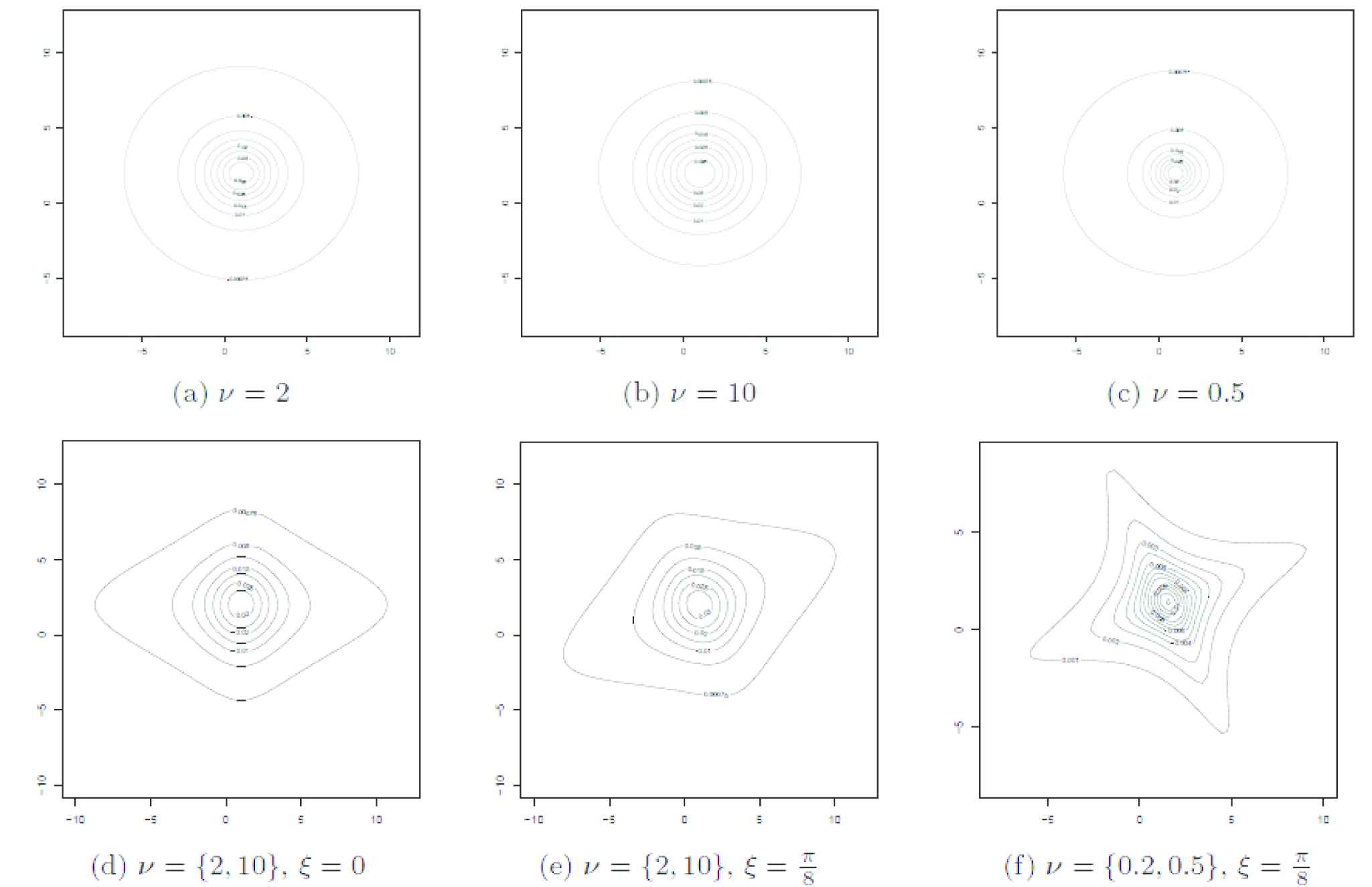
follows one of the distributions below depending on the choice of fwm. For example, setting fwm(wm,θm) to a Gamma distribution T(wm,αm,γm) results in a multivariate generalization of a Pearson type VII distribution. Setting fwm(wm,θm) to T(wm,υm2,υm2) leads to a generalization of the multivariate t–distribution. In Figure 1, we show some of the different shapes in a two-dimensional setting for different values of υ and D, with A fixed to diag(4,4) and μ to (1,2)′ Additional examples are shown in Figure 1 of the Supplementary Materials).
Figure 1
Contour plots of bivariate t–distributions with A=diag(4,4) and μ=(1,2)′.
2.1. An Asymptotic Test
We can write X~=(X1W1,X1W2,…,X1WM)′ a vector of M independent variables X~m whose distributions are given by
∫0∞Nxm,0,1wmfwm(wm)dwm.
In the t-distribution and Pearson VII distribution cases, X~m follows respectively a standard one-dimensional (1D) t-distribution S(xm,0,1wm) and a standard 1D Pearson VII distribution pxm,0,αm,γm. In the t-distribution case, a 1D marginal is then a linear combination of standard 1D t–distributions for which in the general case no closed-form expression is available. However an efficient algorithm to compute such pdfs can be derived according to Witkovsk´y [30]. The derivation in Witkovsk´y [30] is based on the inversion formula of the characteristic function which in the univariate case is
We use the tdist R package of V. Witkovsky available at http://aiolos.um.savba.sk/~viktor/software.html to plot the pdf of some marginals and compare it with 1D t–distributions. We also plot the histogram obtained by simulations to illustrate its consistency with the marginal pdf formula. The fact that the marginals are not in general t–distributions is a notable difference with other multivariate t generalizations. With paying attention to the family of multivariate distribution, we partition the random vector Xi into 1≤ki≤p−1 components as Xi′=X1(i)′,X2(i)′,…,Xki(i)′′, where Xv(i)′∈Rpv(i), p1(i),p2(i),…,pki(i) and p=∑v=1kipv(i). Similarly, the mean vector μi and the covariance matrix Σi are partitioned as μi′=μ1(i)′,μ2(i)′,…,μki(i)′′ and Σi=Σl×m(i)ki×ki, where Σl×m(i)=covXl(i),Xm(i) is the (l×m) th partition of covariance matrix Σi respectively.
Knowing these conventions, the preferred null hypothesis H0 in this paper is that the components X1(i),X2(i),…,Xki(i) are mutually independently distribution, i.e. the density of Xi can be written as the product of the density functions of X1(i),X2(i),…,Xki(i). When we fix the last density, therefore, H0 can be expressed as
Testing H0′ against H1′ is a two-sided test. This test can be done using different methods when the mean vectors and covariance matrices are unknown. To do this, let xi1,xi2,…,xini be the observations on the vector Xi, i=1,2,…,k. Then, the likelihood function of the observed data is given by
where Si=∑j=1nixij−x¯i(xij−x¯)′=Sl×m(i)ki×ki, i=1,2,…,k. It is easy to see that, under the hypothesis H0′ given in (4), the covariance matrix Σi is equal to the diagonal matrix ΣiH0′ with diagonal elements Σ11(i),Σ22(i),…,Σki×ki(i). Therefore, under the null hypothesis, we have
Note that, the statistic Λ in (5) only exists when the inequality min1≤i≤k−1ni>p holds. Here, we suppose that min1≤i≤k−1ni>p+1. By the general theory of Λ's, it is demonstrated that the null distribution of −2logΛ is a chi-squared distribution with df=12(p2−∑v=1k∑r=1ki−1pv(i)2) degrees of freedom as min1≤i≤k−1ni goes to infinity and the dimension is fixed.
andσn=∑i=1kdni−1,p2−2∑v=1kidni−1,pv(i)2ni2n24, n=∑i=1kniandda,b2=log(1+b2a), if the conditionsni>p+1=p1(i)+p2(i)+⋯+pki(i)+1and the fractionpv(i)nigoes tobv(i), where0<bv(i)<1, as the dimension goes to∞fori=1,2,…,ki∈N, hold.
The part (a) holds for the term
NMx,μ,DΔwAD′=∏m=1MN1D′xm;D′xmAmwm−1,
whereAmthemth diagonal element of the diagonal matrixA.
Proof
First, from Hardy et al. [31], if real numbers l1,l2,…,lq are greater than −1, and are all positive or all negative, then we have log∏i=1m(1+li)−log−1+∑i=1mli>0. For given i, i=1,2,…,k, and taking li=−pv(i)ni−1 and m=ki, we see that
For tM(x,μ,Σ,υ) the fraction nin converges to the fraction bbi∈(0,1) as the dimension goes to infinity. In fact, for the second case, bv(i)∈(0,1), the limit is obviously +∞ since lima→1−log(1−a)=−∞. Now fix the value s such that |s|<σ2b and set t=tn=snσn.
It is easy to see that the fraction −nσn2(p+1) converges to the fraction −σ2b<s as the dimension goes to ∞. Then with the fact that
max1≤i≤k12ni<1p+1,
or max1≤i≤kp2ni−1<−1p+1<−12(p+1).
Putting t=tn=snσn>max1≤i≤k{pni−1} as the dimension goes to infinity. Now, for fix i which bi<1, we have dni−1,p2σn2 converge to −log(1−bi)σn2 for max1≤i≤kbi<1 and 0 for max1≤i≤kbi=1. This results that, dni−1,pσn converge to −log(1−bi)σ2 for max1≤i≤kbi<1 and 0 for max1≤i≤kbi=1.
Furthermore, when bi=1, for p–dimensional t–distribution, we have that
2σn2≥dni−1,p2−∑v=1kidni−1,pv(i)2nin2,
if and only if
dni−1,pσn≤2nin2+σn−2∑v=1kidni−1,pv(i)2,
convergence to the fraction 22b<∞ as the dimension goes to ∞. For the density function
px,μ,Σ,θ=∫0∞…∫0∞NMx,μ,DΔwAD′fww1,…,wM;θdw1,…,dwM,
which w1,…,wM are real values, the inequality 2σn2≥(dni−1,p2−∑v=1kidni−1,pv(i)2)(nin)2 also holds. Therefore, from limsupp→∞dni−1,p2σn<∞, we have that 12σn=O(1dni−1,p) or tni2=s2nin1σn=O(1)1σn=O(1dni−1,p). Similarly, since for a<1, the term −log(1−a) is an increasing function, then rni−1,pv(i)2<rni−1,p2. As a result, from limsupp→∞dni−1,pr(i)2σn<limsupp→∞dni−1,p2σn<∞, we have that
12σn=O1dni−1,pv(i),
therefore tni2=O(1dni−1,p). Using the theorem (11.2.3) from Muirhead [32], when the hypothesis H0′ is true, the tth moment of likelihood ratio test given in (4) is
where for complex number z with Re(z)>12(p−1), the multivariate gamma function (Muirhead [32], p. 62) Γp(z)=πp(p−1)2∏j=1pΓ(z−12(j−1)).
Obviously, the expectation (3) only exists when (3ni−12+nit2)>p−12, i=1,2,…,k or t>max1≤i≤k{pni−1}. Recalling t=tn=snσn>max1≤i≤k{pni−1}, tni2=O(1dni−1,p) and tni2=O(1dni−1,pv(i)) as the dimension goes to infinity, by Lemma 5.4 from Jiang and Yang [14], we obtain
as the dimension goes to infinity. Also, we get that
logEexplogΛnσn2s=loge32s2+θn2nσn2s+o(1),
if and only if logE[exp{logΛ−θnnσn2s}]=e12s2+o(1) as dimension goes to infinity. On the other hand, the random variable logΛ−θnnσn2 converges in distribution to standard normal distribution as the dimension goes to infinity and this completes the proof.
The proof of this part is similar to the part (a).
4. COMPARE THE PERFORMANCE OF TESTS
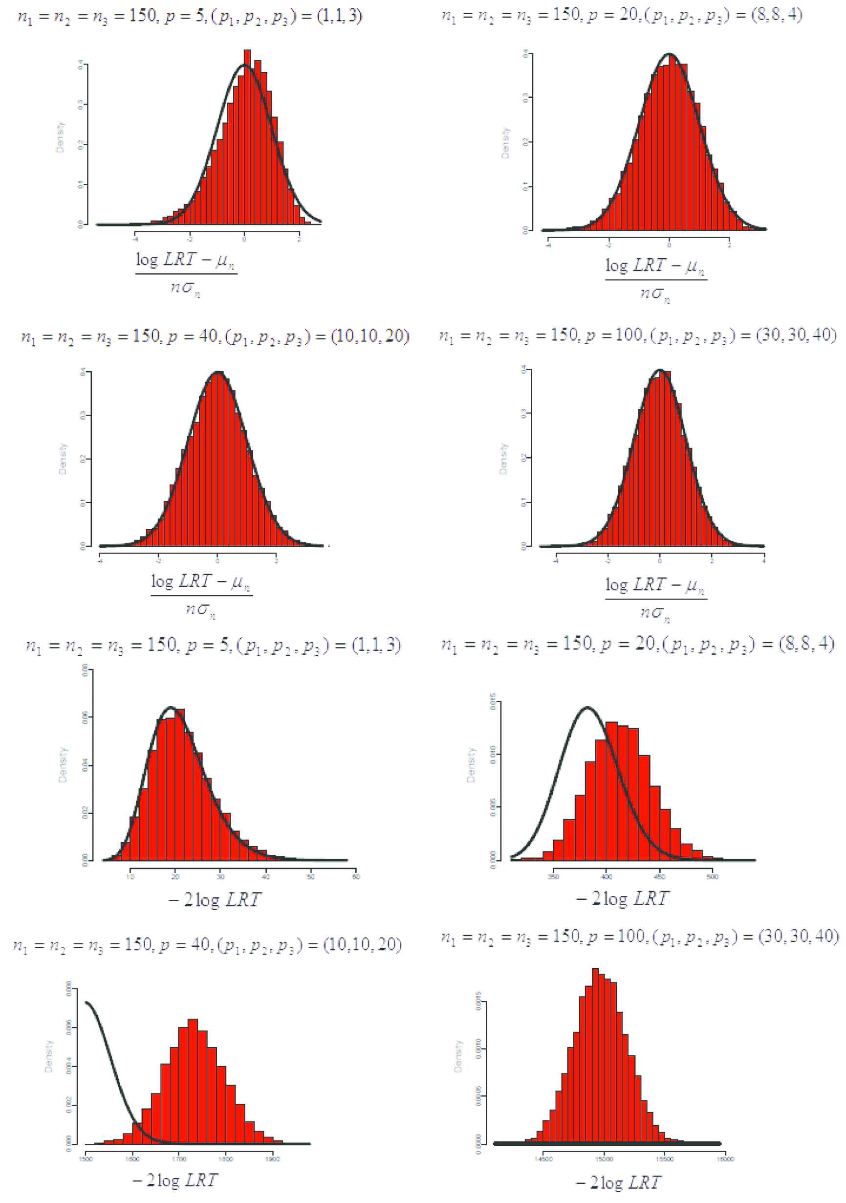
In this section, we compare the performance of the chi-square approximation and normal approximation through a finite sample simulation study. We plot the histograms for the chi-square statistics which are used for the chi-square approximation and compare with their corresponding limiting chi-square curves. In this simulation, the notation Kp stands for the p×p matrix whose entries are all equal to 1, and Ip is equal to an p×p identity matrix. Also, without loss of generality, we suppose that all the population covariance matrices Σi's are equal to ρKp+(1−ρ)Ip with 0≤ρ≤1, mean vectors θi's are all equal to zero, the nominal Type I error rate α is 0.05 and k=3. Furthermore, we consider the same partition of p for all k distributions. For each combination of ρ, n1, n2, n3 and p, using 20000 replications from the multivariate normal distribution Np0,ρKp+(1−ρ)Ip, with mean vector 0, the simulated values of size, H0′, and power with ρ>0, for chi-square and normal approximations are calculated and given in Tables 1 and 2. Also, in Figure 2, for different values of simulation parameters, the histograms of 20000 simulated null values of logΛ−θnnσn2 and −2logΛ with added standard normal and chi-square curves are pictures, respectively. We choose k=3, n1=n2=n3=150 and p=5,20,40,100, with same partition of p for each of the k distribution as (p1,p2,p3)=(1,1,3) for p=5, (p1,p2,p3)=(8,8,4) for p=20, (p1,p2,p3)=(10,10,20) for p=40, and (p1,p2,p3)=(30,30,40) for p=100.
ρ
(n1,n2,n3)
p
Partition of p
Size under H0′ Chi-square Approximation
Size under H0′ Normal Approximation
(25,25,25)
5
2, 1, 2
0.454
0.038
0
(25,25,25)
10
4, 3, 3
0.761
0.042
(25,25,25)
20
4, 5, 6, 5
0.923
0.052
(50,50,50)
5
2, 3
0.389
0.047
0
(50,50,50)
20
5, 7, 8
0.636
0.051
(50,50,50)
45
17, 15, 13
0.801
0.061
(100,100,100)
5
3, 2
0.266
0.046
0
(100,100,100)
50
15, 17, 18
0.745
0.050
(100,100,100)
95
15, 30 30, 20
0.922
0.055
(150,150,150)
5
1, 4
0.257
0.042
0
(150,150,150)
50
12, 24, 13, 21, 10
0.481
0.054
(150,150,150)
95
50, 70, 25
0.792
0.054
Table 1
The simulated values of size for two tests under H0′.
ρ
(n1,n2,n3)
p
Partition of p
Power under H1′ Chi-square Approximation
Power under H1′ Normal Approximation
(25,25,25)
5
2, 1, 2
0.750
0.895
0.05
(25,25,25)
10
4, 3, 3
0.739
0.812
(25,25,25)
20
4, 5, 6, 5
0.634
0.730
(50,50,50)
5
2, 3
0.743
0.927
0.05
(50,50,50)
20
5, 7, 8
0.694
0.804
(50,50,50)
45
17, 15, 13
0.605
0.729
(100,100,100)
5
2, 3
0.811
0.965
0.05
(100,100,100)
20
15, 17, 18
0.669
0.914
(100,100,100)
45
15, 30, 30, 20
0.504
0.823
(150,150,150)
5
1, 4
0.693
0.874
0.05
(150,150,150)
20
12, 24, 13, 21, 10
0.610
0.751
(150,150,150)
45
50, 70, 25
0.592
0.714
(25,25,25)
5
2, 1, 2
0.653
0.870
0.6
(25,25,25)
10
4, 3, 3
0.624
0.813
(25,25,25)
20
4, 5, 6, 5
0.548
0.685
(50,50,50)
5
2, 3
0.785
0.925
0.6
(50,50,50)
10
5, 7, 8
0.624
0.824
(50,50,50)
20
17, 15, 13
0.603
0.741
(100,100,100)
5
2, 3
0.764
0.873
0.6
(100,100,100)
10
15, 17, 18
0.525
0.745
(100,100,100)
20
15, 30, 30, 20
0.511
0.655
(150,150,150)
5
1, 4
0.745
0.843
0.6
(150,150,150)
80
12, 24, 13, 21, 10
0.603
0.771
(150,150,150)
145
50, 70, 25
0.590
0.723
Table 2
The simulated values of power for two tests under H1′.
Figure 2
The histogram of simulated null values of logΛ−θnnσn2 and −2logΛ.
The plots in the top row of Figure 2 indicate that logΛ−θnnσn2 and standard normal curve match better as the dimension becomes larger and the pictures in the bottom row show that the histogram of −2logΛ move away gradually from chi-square curve as the dimension grows.
From Tables 1 and 2, we inference that our normal approximation and the classical chi-square approximation are comparable for the large sample sizes and small values of dimension. Under the hypothesis H0′, by increasing the dimension, the simulated size chi-square approximation tends to one, whereas the simulated size of the our proposed method is around 0.05.
From Table 2, we see that the power of normal approximation is greater than the power of chi-square approximation and also for any fixed sample sizes, by increasing the dimension, the power of our normal approximation decreases.
5. CONCLUDING REMARKS
In this paper, an asymptotic two-sided test in a family of multivariate distribution components with mean vector and positive definite matrix was considered. Using the likelihood ratio method a test statistic computed and the asymptotic distribution proposed. We studied the distribution approximation computed using the likelihood ratio test and an efficient algorithm to compute the density functions can be derived according to Witkovsk´y [30]. Also, a simulation study presented on the sample sizes and powers to show that the proposed distribution approximation outperform the classical distribution approximation.
CONFLICT OF INTEREST
There is no conflict of interest to declare.
ACKNOWLEDGMENTS
The authors gratefully thank to Editor in chief and the referees for their constructive comments and recommendations which definitely help to improve the readability and quality of the paper.
TY  - JOUR
AU  - Abouzar Bazyari
AU  - Mahmoud Afshari
AU  - Monjed H. Samuh
PY  - 2020
DA  - 2020/05/26
TI  - An Asymptotic Two-Sided Test in a Family of Multivariate Distribution
JO  - Journal of Statistical Theory and Applications
SP  - 162
EP  - 172
VL  - 19
IS  - 2
SN  - 2214-1766
UR  - https://doi.org/10.2991/jsta.d.200511.001
DO  - 10.2991/jsta.d.200511.001
ID  - Bazyari2020
ER  -